An Efficient K-Means Clustering Algorithm
Khaled Alsabti
Syracuse University
Sanjay Ranka
University of Florida
Vineet Singh
Hitachi America, Ltd.
Abstract
In this paper, we present a novel algorithm for perform-ing k-means clusterperform-ing. It organizes all the patterns in a k-d tree structure such that one can find all the patterns which are closest to a given prototype efficiently. The main intu-ition behind our approach is as follows. All the prototypes are potential candidates for the closest prototype at the root level. However, for the children of the root node, we may be able to prune the candidate set by using simple geometrical constraints. This approach can be applied recursively until the size of the candidate set is one for each node.
Our experimental results demonstrate that our scheme can improve the computational speed of the direct k-means algorithm by an order to two orders of magnitude in the total number of distance calculations and the overall time of computation.
1. Introduction
Clustering is the process of partitioning or grouping a given set of patterns into disjointclusters. This is done such that patterns in the same cluster are alike and patterns be-longing to two different clusters are different. Clustering has been a widely studied problem in a variety of applica-tion domains including neural networks, AI, and statistics.
Several algorithms have been proposed in the literature for clustering: ISODATA [8, 3], CLARA [8], CLARANS [10], Focusing Techniques [5] P-CLUSTER [7]. DBSCAN [4], Ejcluster [6], BIRCH [14] and GRIDCLUS [12].
The k-means method has been shown to be effective in producing good clustering results for many practical appli-cations. However, a direct algorithm of k-means method requires time proportional to the product of number of pat-terns and number of clusters per iteration. This is computa-tionally very expensive especially for large datasets.
We propose a novel algorithm for implementing the k-means method. Our algorithm produces the same or
com-✁
This work was supported by the Information Technology Lab (ITL) of Hitachi America, Ltd. while K. Alsabti and S. Ranka were visiting ITL.
parable (due to the round-off errors) clustering results to the direct k-means algorithm. It has significantly superior per-formance than the direct k-means algorithm in most cases.
The rest of this paper is organized as follows. We review previously proposed approaches for improving the perfor-mance of the k-means algorithms in Section 2. We present our algorithm in Section 3. We describe the experimental results in Section 4 and we conclude with Section 5.
2
k-means Clustering
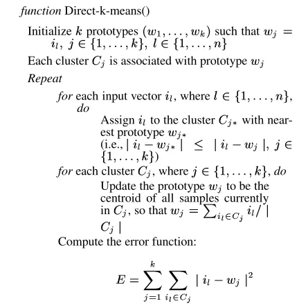
In this section, we briefly describe the direct k-means algorithm [9, 8, 3]. The number of clusters
✂
is assumed to be fixed in k-means clustering. Let the
✂
prototypes ✄✆☎✞✝✠✟☛✡☛✡☞✡✌✟✍☎✏✎✒✑
be initialized to one of the ✓ input patterns ✄✆✔✍✝✕✟☞✡☛✡☞✡☛✟✍✔✗✖✘✑
.1 Therefore,
☎✚✙✞✛✜✔✣✢✗✟✥✤✧✦✩★✫✪✬✟☞✡☛✡☛✡☛✟ ✂✮✭
✟✰✯✱✦✲★✒✪✬✟☞✡☛✡☞✡✳✟
✓
✭
Figure 1 shows a high level description of the direct k-means clustering algorithm. ✴
✙
is the
✤
th cluster whose value is a disjoint subset of input patterns. The quality of the clustering is determined by the following error function:
✵
✛
✎
✶
✙✸✷ ✝
✶
✹✻✺✽✼✬✾❀✿✏❁ ✔✣✢✮❂❃☎✚✙
❁❄
The appropriate choice of✂
is problem and domain de-pendent and generally a user tries several values of
✂
. As-suming that there are✓ patterns, each of dimension❅ , the computational cost of a direct k-means algorithm per itera-tion (of the repeat loop) can be decomposed into three parts:
1. The time required for the first forloop in Figure 1 is
❆
✄
✓
✂
❅
✑
.
2. The time required for calculating the centroids (second forloop in Figure 1) is
❆ ✄ ✓❇❅
✑
.
3. The time required for calculating the error function is
❆
✄
✓❇❅
✑
.
The number of iterations required can vary in a wide range from a few to several thousand depending on the number of patterns, number of clusters, and the input data distribution. Thus, a direct implementation of the k-means method can be computationally very intensive. This is es-pecially true for typical data mining applications with large number of pattern vectors.
functionDirect-k-means()
Initialize prototypes ✁✄✂✆☎✞✝✠✟✠✟✡✟✠✝☛✂✌☞✎✍ such that✂✑✏✓✒ ✔✖✕
✝✘✗✚✙✜✛✣✢✎✝✞✟✠✟✠✟✡✝ ✥✤
✝✧✦★✙✩✛✣✢✎✝✞✟✠✟✡✟✠✝✫✪
✤
Each cluster✬✧✏ is associated with prototype✂✭✏
Repeat
foreach input vector✔✮✕
, where✦✯✙✰✛✣✢✎✝✞✟✞✟✠✟✡✝✫✪
✤
,
do
Assign✔✖✕
to the cluster✬✱✏
✁ with
near-Update the prototype✂✯✏ to be the
centroid of all samples currently in✬✧✏ , so that✂✯✏✻✒✽✼✿✾
✺❁❀✺❂✒✿ ✔✖✕✄❃
✲
✬✧✏❄✲
Compute the error function:
❅
does not change significantly or cluster mem-bership no longer changes
Figure 1. Direct k-means clustering algorithm
There are two main approaches described in the litera-ture which can be used to reduce the overall computational requirements of the k-means clustering method especially for the distance calculations:
1. Use the information from the previous iteration to reduce the number of distance calculations. P-CLUSTER is a k-means-based clustering algorithm which exploits the fact that the change of the assign-ment of patterns to clusters are relatively few after the first few iterations [7]. It uses a heuristic which deter-mines if the closest prototype of a pattern❊ has been changed or not by using a simple check. If the assign-ment has not changed, no further distance calculations are required. It also uses the fact that the movement of the cluster centroids is small for consecutive iterations (especially after a few iterations).
2. Organize the prototype vectors in a suitable data struc-ture so that finding the closest prototype for a given
pattern becomes more efficient [11, 13]. This prob-lem reduces to finding the nearest neighbor probprob-lem for a given pattern in the prototype space. The number of distance calculations using this approach is propor-tional to✓●❋■❍
per iteration. For many applica-tions such as vector quantization, the prototype vectors are fixed. This allows for construction of optimal data structures to find the closest vector for a given input test pattern [11]. However, these optimizations are not applicable to the k-means algorithm as the prototype vectors will change dynamically. Further, it is not clear how these optimizations can be used to reduce the time for calculation of the error function (which becomes a substantial component after reduction in the number of distance calculations).
3
Our Algorithm
The main intuition behind our approach is as follows. All the prototypes are potential candidates for the closest prototype at the root level. However, for the children of the root node, we may be able to prune the candidate set by using simple geometrical constraints. Clearly, each child node will potentially have different candidate sets. Further, a given prototype may belong to the candidate set of several child nodes. This approach can be applied recursively till the size of the candidate set is one for each node. At this stage, all the patterns in the subspace represented by the subtree have the sole candidate as their closest prototype. Using this approach, we expect that the number of distance calculation for the first loop (in Figure 1) will be propor-tional to ✓❏❋▲❑
is much smaller than
❍
. This is because the distance calculation has to be performed only with internal nodes (representing many pat-terns) and not the patterns themselves in most cases. This approach can also be used to significantly reduce the time requirements for calculating the prototypes for the next it-eration (second for loop in Figure 1). We also expect the time requirement for the second for loop to be proportional to✓▲❋▼❑
✄✂ ✟
❅
✑
.
The improvements obtained using our approach are cru-cially dependent on obtaining good pruning methods for ob-taining candidate sets for the next level. We propose to use the following strategy.
◆
For each candidate
☎
✹
, find the minimum and maxi-mum distances to any point in the subspace
◆
Find the minimum of maximum distances, call it
❖
✔
✓
❖◗P✴❘
◆
Prune out all candidates with minimum distance greater than❖
✔
✓
The above strategy guarantees that no candidate is pruned if it can potentially be closer than any other candidate pro-totype to a given subspace.
Our algorithm is based on organizing the pattern vectors so that one can find all the patterns which are closest to a given prototype efficiently. In the first phase of the algo-rithm, we build a k-d tree to organize the pattern vectors. The root of such a tree represents all the patterns, while the children of the root represent subsets of the patterns com-pletely contained in subspaces (Boxes). The nodes at the lower levels represent smaller boxes. For each node of the tree, we keep the following information:
1. The number of points ( )
2. The linear sum of the points ( ✁✄✂
Let the number of dimensions be❅ and the depth of the k-d tree be ✟ . The extra time and space requirements for maintaining the above information at each node is propor-tional to❆
✄
✓❇❅
✑
.2 Computing the medians at
✟ levels takes time❆
✄
✓✠✟
✑
[2]. These set of medians are needed in per-forming the splitting of the internal nodes of the tree. There-fore, the total time requirement for building this tree such that each internal node at a given level represents the same number of elements is
❆ ✄
For building the k-d tree, there are several competing choices which affect the overall structure.
1. Choice of dimension used for performing the split: One option is to choose a common dimension across all the nodes at the same level of the tree. The dimen-sions are chosen in a round-robin fashion for different levels as we go down the tree. The second option is to use the splitting dimension with the longest length.
2. Choice of splitting point along the chosen dimension: We tried two approaches based on choosing the central splitting point or median splitting point. The former di-vides the splitting dimensions into two equal parts (by width) while the latter divides the dimensions such that there are equal number of patterns on either side. We will refer to these approaches as midpoint-based and median-based approaches respectively. Clearly, the cost of the median-based approach is slightly higher as it requires calculation of the median.
We have empirically investigated the effect of the two choices on the overall performance of our algorithms.
2The same information (
✌ ,✍✏✎ ,✎✑✎ ) has also been used in [14] and is
calledClustering Feature(CF). However, as we will see later, we use CF in a different way.
3For the rest of the paper, patterns and points are used interchangeably.
These results show that splitting along the longest dimen-sion and choosing a midpoint-based approach for splitting is preferable [1].
In the second phase of the k-means algorithm, the ini-tial prototypes are derived. Just as in the direct k-means algorithm, these initial prototypes are generated randomly or drawn from the dataset randomly.4
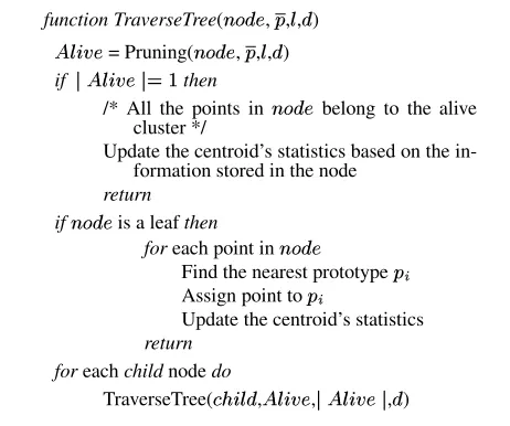
function TraverseTree(✪✓✒✕✔✗✖ ,✘ ,✦,✔ )
/* All the points in✪✓✒✜✔✗✖ belong to the alive
cluster */
Update the centroid’s statistics based on the in-formation stored in the node
return if✪✓✒✜✔✗✖ is a leafthen
foreach point in✪✢✒✕✔✗✖
Find the nearest prototype✘
✾
Assign point to✘
✾
Update the centroid’s statistics
return foreachchildnodedo
TraverseTree(✣✥✤
Figure 2. Tree traversal algorithm
In the third phase, the algorithm performs a number of it-erations (as in the direct algorithm) until a termination con-dition is met. For each cluster
✔
, we maintain the number of points✴
✹
✖
, the linear sum of the points✴
✹
✧✢★ and the square sum of the points✴
✹
★✩★ .
In each iteration, we traverse the k-d tree using a depth-firststrategy (Figure 2) as follows.5 We start from the root node with all
✂
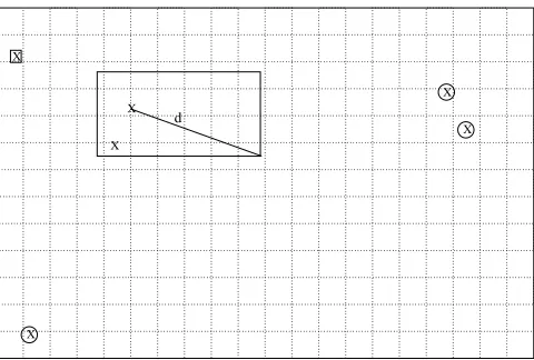
candidate prototypes. At each node of the tree, we apply a pruning function on the candidates proto-types. A high level description of the pruning algorithm is given in Figure 3. If the number of candidate prototypes is equal to one, the traversal below that internal node is not pursued. All the points belonging to this node have the sur-viving candidate as the closest prototype. The cluster statis-tics are updated based on the information about the number of points, linear sum, and square sum stored for that inter-nal node. A direct k-means algorithm is applied on the leaf node if there is more than one candidate prototype. This di-rect algorithm performs one iteration of the didi-rect algorithm on the candidate prototypes and the points of the leaf node. An example of the pruning achieved by using our algo-rithm is shown in Figure 4. Our approach is a conservative
4The k-d tree structure can potentially be used to derive better
ap-proaches for this choice. However, these have not been investigated in this paper.
function Pruning(✂✁☎✄✝✆✟✞
foreach prototype✘
✾
✙ ✘ do
Compute the minimum (✠
✔
✪
✾) and maximum
(✠☛✡✌☞
✾) distances for any point in the box
representing the✂✁☎✄✝✆✟✞ ✖ ✖
Find the minimum of✠✍✡✌☞
✾ ✎✑✏☛✒
foreach prototype✘
✾
Figure 3. Pruning algorithm
approach and may miss some of the pruning opportunities. For example, the candidate shown as an x with a square around it could be pruned with a more complex pruning strategy. However, our approach is relatively inexpensive and can be shown to require time proportional to
✂
. Choos-ing a more expensive prunChoos-ing algorithm may decrease the overall number of distance calculations. This may, how-ever, be at the expense of higher overall computation time due to an offsetting increase in cost of pruning.
X
Figure 4. Example of pruning achieved by our algorithm. X represents the candidate set. ❅ is the MinMax distance. All the candidates which are circled get pruned. The candidate with a square around it is not pruned by our algorithm
At the end of each iteration, the new set of centroids is derived and the error function is computed as follows.
1. The new centroid for cluster
✔
is: ✾✢✜
✣✌✤ ✾ ✜
2. The error function is: ✼
✹
The leaf size is an important parameter for tuning the overall performance of our algorithm. Small leaf size re-sults in larger cost for constructing the tree, and increases the overall cost of pruning as the pruning may have to be continued to lower levels. However, a small leaf size de-creases the overall cost for distance calculations for finding the closest prototype.
Calculating the Minimum and Maximum Distances
The pruning algorithm requires calculation of the minimum as well as maximum distance to any given box from a given prototype. It can be easily shown that the maximum dis-tance will be to one of the corners of the box. Let❍✮✭✰✯✲✱✴✳✰✵✲✶✷✱
✹
be that corner for prototype
✔
(✝
✹
). The coordinates of
❍✮✭✰✯✲✱✴✳✰✵✪✶✸✱ be computed as follows:
❍✮✭✮✯✺✱✴✳✰✵✪✶✷✱
are the lower and upper coordinates of the box along dimension
✤
.
The maximum distance can be computed as follows:
❅
A naive approach for calculating maximum and mini-mum distances for each prototype will perform the above calculations for each node (box) of the tree indpenedently; which will require❆
✄
❅
✑
time. The coordinates of the box of the child node is exactly the same as its parent except for one dimension which has been used for splitting at the parent node. This information can be exploited to reduce the time to constant time. This requires the use of the max-imum distance of the prototype to the parent node. This can be used to express the maximum square distance for the child node in terms of its parent. The computation cost of the above approach is
❆ ✄✍✪ ✑
for each candidate prototype. The overall computational requirement for a node with
✂
candidate prototypes is ❆ ✄✂ ✑
. The value of minimum dis-tance can be obtained similarly. For more details the reader is referred to a detailed version of this paper [1].
4
Experimental Results
ex-perimental results reported are on a IBM RS/6000 running AIX version 4. The clock speed of the processor is 66 MHz and the memory size is 128 MByte.
For each dataset and the number of clusters, we com-pute the factors ❑ ✟ and ❑
✂✁
of reduction in distance calculations and overall execution time over the direct algo-rithm respectively as well as the average number of distance calculations per pattern✄ ✟ ✴ . The number of distance cal-culations for the direct algorithm is
✄✂
✡
✪✕✑
✓ per iteration.
6
All time measurements are in seconds.
Our main aim in this paper is to study the computational aspects of the k-means method. We used several datasets all of which have been generated synthetically. This was done to study the scaling properties of our algorithm for different values of✓ and
✂
respectively. Table 1 gives a description for all the datasets. The datasets used are as follows:
1. We used three datasets (DS1, DS2 and DS3). These are described in [14].
2. For the datasets R1 through R12, we have generated✂ points randomly in a cube of appropriate dimensional-ity. For the
✔
th point we generate
✔
❄
✖
✦
✎✆☎✰✝
✩
✎
points around it using uniform distribution. These result in clusters with non-uniform number of points.
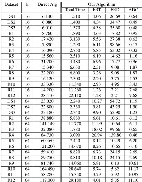
We experimented with leaf sizes of 4, 16, 64 and 256. For most of our datasets, we found that choosing a leaf size of 64 resulted in optimal or near optimal performance. Fur-ther, the overall performance was not sensitive to the leaf size except when the leaf size was very small.
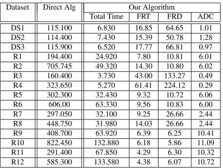
Tables 2 and 3 present the performance of our algorithms for different number of clusters and iterations assuming a leaf size of 64. For each combination used, we present the factor reduction in overall time (FRT) and the time of the direct k-means algorithm. We also present the factor reduction in distance calculations (FRD) and the average number of distance calculations per pattern (ADC). These results show that our algorithm can improve the overall per-formance of k-means clustering by an order to two orders of magnitude. The average number of distance calculations required is very small and can vary anywhere from 0.17 to 11.17 depending on the dataset and the number of clusters required.
The results presented in [7] show that their methods re-sult in factor of 4 to 5 improvements in overall compu-tational time. Our improvements are substantially better. However, we note that the datasets used are different and a direct comparison may not be accurate.
6This includes the
✝✜✌ distance calculations for finding the nearest
pro-totype and the equivalent of✌ distance calculations for computing he new
set of centroids.
Dataset k Direct Alg Our Algorithm
Total Time FRT FRD ADC DS1 16 6.140 1.510 4.06 26.69 0.64 DS2 16 6.080 1.400 4.34 34.47 0.49 DS3 16 6.010 1.370 4.38 35.68 0.48 R1 16 8.760 1.890 4.63 17.82 0.95 R2 16 17.420 3.130 5.56 27.38 0.62 R3 16 7.890 1.290 6.11 98.66 0.17 R4 16 16.090 2.750 5.85 53.02 0.32 R5 16 15.560 2.510 6.19 14.62 1.16 R6 16 31.200 4.480 6.96 17.77 0.96 R7 16 15.340 6.630 2.31 9.08 1.87 R8 16 22.200 6.800 3.26 9.08 1.87 R9 16 16.120 7.300 2.20 3.75 4.53 R10 16 33.330 11.340 2.93 4.96 3.43 R11 16 14.200 11.260 1.26 2.21 7.68 R12 16 28.410 22.110 1.28 2.21 7.68 DS1 64 23.020 2.240 10.27 54.72 1.19 DS2 64 22.880 2.330 9.81 43.25 1.50 DS3 64 23.180 2.340 9.90 52.90 1.23 R1 64 38.880 5.880 6.61 10.61 6.12 R2 64 141.149 11.770 11.99 10.64 6.11 R3 64 32.080 1.780 18.02 99.66 0.65 R4 64 64.730 3.090 20.94 139.80 0.46 R5 64 60.460 7.440 8.12 10.49 6.20 R6 64 121.200 14.670 8.26 10.65 6.10 R7 64 59.410 8.820 6.73 24.15 2.69 R8 64 89.750 8.810 10.18 24.15 2.69 R9 64 81.740 14.060 5.81 6.13 10.61 R10 64 164.490 28.640 5.74 5.82 11.17 R11 64 58.280 15.340 3.79 5.92 10.97 R12 64 117.060 29.180 4.01 5.85 11.10
Table 2. The overall results for 10 iterations
5
Conclusions
In this paper, we presented a novel algorithm for per-forming k-means clustering. Our experimental results demonstrated that our scheme can improve the direct k-means algorithm by an order to two orders of magnitude in the total number of distance calculations and the overall time of computation.
There are several improvements possible to the basic strategy presented in this paper. One approach will be to restructure the tree every few iterations to further reduce the value of❑
✄ ✂ ✟
❅
✑
Dataset Size Dimensi- No. of Characteristic Range onality Clusters
DS1 100,000 2 100 Grid [-3,41]
DS2 100,000 2 100 Sine [2,632],[-29,29] DS3 100,000 2 100 Random [-3,109],[-15,111]
R1 128k 2 16 Random [0,1]
R2 256k 2 16 Random [0,1]
R3 128k 2 128 Random [0,1]
R4 256k 2 128 Random [0,1]
R5 128k 4 16 Random [0,1]
R6 256k 4 16 Random [0,1]
R7 128k 4 128 Random [0,1]
R8 256k 4 128 Random [0,1]
R9 128k 6 16 Random [0,1]
R10 256k 6 16 Random [0,1]
R11 128k 6 128 Random [0,1]
R12 256k 6 128 Random [0,1]
Table 1. Description of the datasets. The range along each dimension is the same unless explicitly stated
Dataset Direct Alg Our Algorithm
Total Time FRT FRD ADC DS1 115.100 6.830 16.85 64.65 1.01 DS2 114.400 7.430 15.39 50.78 1.28 DS3 115.900 6.520 17.77 66.81 0.97 R1 194.400 24.920 7.80 10.81 6.01 R2 705.745 49.320 14.30 10.80 6.02 R3 160.400 3.730 43.00 133.27 0.49 R4 323.650 5.270 61.41 224.12 0.29 R5 302.300 32.430 9.32 10.72 6.06 R6 606.00 63.330 9.56 10.83 6.00 R7 297.050 32.100 9.25 26.66 2.44 R8 448.750 31.980 14.03 26.66 2.44 R9 408.700 63.920 6.39 6.25 10.41 R10 822.450 132.880 6.18 5.86 11.09 R11 291.400 67.850 4.29 6.30 10.32 R12 585.300 133.580 4.38 6.07 10.72
Table 3. The overall results for 50 iterations and 64 clusters
References
[1] K. Alsabti, S. Ranka, and V. Singh. An Efficient K-Means Clustering Algorithm. http://www.cise.ufl.edu/ ranka/, 1997.
[2] T. H. Cormen, C. E. Leiserson, and R. L. Rivest. Introduc-tion to Algorithms. McGraw-Hill Book Company, 1990. [3] R. C. Dubes and A. K. Jain.Algorithms for Clustering Data.
Prentice Hall, 1988.
[4] M. Ester, H. Kriegel, J. Sander, and X. Xu. A Density-Based Algorithm for Discovering Clusters in Large Spatial Databases with Noise.Proc. of the 2nd Int’l Conf. on Knowl-edge Discovery and Data Mining, August 1996.
[5] M. Ester, H. Kriegel, and X. Xu. Knowledge Discovery in Large Spatial Databases: Focusing Techniques for Efficient
Class Identification.Proc. of the Fourth Int’l. Symposium on Large Spatial Databases, 1995.
[6] J. Garcia, J. Fdez-Valdivia, F. Cortijo, and R. Molina. Dy-namic Approach for Clustering Data. Signal Processing, 44:(2), 1994.
[7] D. Judd, P. McKinley, and A. Jain. Large-Scale Parallel Data Clustering. Proc. Int’l Conference on Pattern Recognition, August 1996.
[8] L. Kaufman and P. J. Rousseeuw. Finding Groups in Data: an Introduction to Cluster Analysis. John Wiley & Sons, 1990.
[9] K. Mehrotra, C. Mohan, and S. Ranka.Elements of Artificial Neural Networks. MIT Press, 1996.
[10] R. T. Ng and J. Han. Efficient and Effective Clustering Meth-ods for Spatial Data Mining. Proc. of the 20th Int’l Conf. on Very Large Databases, Santiago, Chile, pages 144–155, 1994.
[11] V. Ramasubramanian and K. Paliwal. Fast K-Dimensional Tree Algorithms for Nearest Neighbor Search with Applica-tion to Vector QuantizaApplica-tion Encoding. IEEE Transactions on Signal Processing, 40:(3), March 1992.
[12] E. Schikuta. Grid Clustering: An Efficient Hierarchical Clustering Method for Very Large Data Sets. Proc. 13th Int’l. Conference on Pattern Recognition, 2, 1996.
[13] J. White, V. Faber, and J. Saltzman. United States Patent No. 5,467,110. Nov. 1995.
[14] T. Zhang, R. Ramakrishnan, and M. Livny. BIRCH: An Ef-ficient Data Clustering Method for Very Large Databases.