Contents lists available atScienceDirect
Progress in Oceanography
journal homepage:www.elsevier.com/locate/pocean
Review
Uncertainties and applications of satellite-derived coastal water quality
products
Guangming Zheng
a,b,⁎, Paul M. DiGiacomo
aaNOAA/NESDIS Center for Satellite Applications and Research, 5830 University Research Court, College Park, MD 20740, USA bGlobal Science & Technology, Inc., 7855 Walker Drive, Suite 200, Greenbelt, MD 20770, USA
A R T I C L E I N F O
Keywords: Light absorption Light scattering Light backscattering Water-leaving radiance Remote-sensing reflectance Water quality
Pollutants Pathogens Chlorophyll Suspended particles Suspended sediment
Chromophoric dissolved organic matter
A B S T R A C T
Recent and forthcoming launches of a plethora of ocean color radiometry sensors, coupled with increasingly adopted free and open data policies are expected to boost usage of satellite ocean color data and drive the demand to use these data in a quantitative and routine manner. Here we review factors that introduce certainties to various satellite-derived water quality products and recommend approaches to minimize the un-certainty of a specific product. We show that the regression relationships between remote-sensing reflectance and water turbidity (in terms of nephelometric units) established for different regions tend to converge and therefore it is plausible to develop a global satellite water turbidity product derived using a single algorithm. In contrast, solutions to derive suspended particulate matter concentration are much less generalizable; in one case it might be more accurate to estimate this parameter based on satellite-derived particulate backscattering coefficient, whereas in another the nonagal particulate absorption coefficient might be a better proxy. Regarding satellite-derived chlorophyll concentration, known to be subject to large uncertainties in coastal waters, studies summarized here clearly indicate that the accuracy of classical reflectance band-ratio algorithms depends largely on the contribution of phytoplankton to total light absorption coefficient as well as the degree of correlation between phytoplankton and the dominant nonalgal contributions. Our review also indicates that currently available satellite-derived water quality products are restricted to optically significant materials, whereas many users are interested in toxins, nutrients, pollutants, and pathogens. Presently, proxies or indicators for these constituents are inconsistently (and often incorrectly) developed and applied. Progress in this general direction will remain slow unless, (i) optical oceanographers and environmental scientists start collaborating more closely and make optical and environmental measurements in parallel, (ii) more efforts are devoted to identifying optical, ecological, and environmental forerunners of autochthonous water quality issues (e.g., onsite growth of pathogens), and, (iii) environmental processes associated with the source, transport, and transformation of al-lochthonous issues (e.g., transport of nutrients) are better understood. Accompanying these challenges, the need still exists to conduct fundamental research in satellite ocean color radiometry, including development of more robust atmospheric correction methods as well as inverse models for coastal regions where optical properties of both aerosols and hydrosols are complex.
1. Introduction
Coastal (marine, estuarine, and inland) zones are among the most important and valuable regions in the world from both an ecological and a socio-economic perspective. They are extremely productive, supplying living aquatic (e.g.,fisheries; diverse benthic habitats) and other natural resources (e.g., oil, gas, minerals, and water). They are also hubs of commerce and transportation, and the most heavily po-pulated and urbanized regions on earth. As such, coastal pollution is a significant and growing problem in both developed and developing
nations. Contaminants such as oil, toxic chemicals, heavy metals, bac-teria, viruses, nutrients, and sediments can adversely impact human health and coastal ecosystems and thus have significant environmental and socio-economic ramifications (e.g., Islam and Tanaka, 2004; IOCCG, 2008; Karydis and Kitsiou, 2013).
It can be difficult to identify sources of pollution in coastal zones, as well as monitoring and forecasting the subsequent fate, transport, and impacts of contaminants. In particular, coastal zones are interfacial re-gions where atmospheric, aquatic, and terrestrial domains converge (Karydis and Kitsiou, 2013) and are typically characterized by complex
http://dx.doi.org/10.1016/j.pocean.2017.08.007
Received 12 December 2016; Received in revised form 29 August 2017; Accepted 30 August 2017
⁎Corresponding author at: NOAA/NESDIS Center for Satellite Applications and Research, 5830 University Research Court, College Park, MD 20740, USA. E-mail address:[email protected](G. Zheng).
Available online 01 September 2017
dynamics, including small-scale, ephemeral, and episodic processes and phenomena. Pollution inputs can be localized within one of these do-mains (e.g., an offshore oil spill that does not reach land) or else be trans-boundary in nature (e.g., urban or agricultural runoffdischarged into an ocean or lake, or an offshore oil spill or sewage discharge transported onshore). Pollution sources can also be characterized as either“point”or
“nonpoint”types. Point sources of pollution in the coastal environment are singular and localized and include discharge from a shore-based in-dustrial or municipal wastewater treatment plant, or from a ship or other offshore structure (e.g., oil platform). Nonpoint sources of pollution in the coastal environment come from many diffuse sources and can include stormwater runoffas well as atmospheric deposition.
Nomenclature
Acronyms
AVIRIS Airborne Visible/Infrared Imaging Spectrometer CDOM Chromophoric Dissolved Organic Matter Chl-a Chlorophyll-a
DOC Dissolved Organic Carbon EPA Environmental Protection Agency FIB Fecal Indicator Bacteria
FNRU Formazin Nephelometric Ratio Unit FNU Formazin Nephelometric Unit
GCOM-C Global Change Observation Mission-Climate GEO Group on Earth Observations
GEOSS Global Earth Observation System of Systems GOCI Geostationary Ocean Color Imager
HAB Harmful Algal Bloom
HICO Hyperspectral Imager for the Coastal Ocean IOCCG International Ocean Color Coordinating Group IOP Inherent Optical Property
ISO International Organization for Standardization JPSS Joint Polar Satellite System
MAA Mycosporine-like Amino Acid
MERIS MEdium Resolution Imaging Spectrometer MODIS MODerate-resolution Imaging Spectroradiometer MSI Multi-Spectral Imager
NIR Near-Infrared
NOMAD NASA bio-Optical Marine Algorithm Dataset NTRU Nephelometric Turbidity Ratio Unit NTU Nephelometric Turbidity Unit OCR Ocean Color Radiometry OLCI Ocean and Land Color Instrument OLI Operational Land Imager
PACE Plankton, Aerosol, Cloud, and ocean Ecosystem PSU practical salinity units
RGB Red-Green-Blue (Image) SAR Synthetic Aperture Radar
SeaWiFS Sea-viewing Wide Field-of-view Sensor
SeaBASS SeaWiFS Bio-optical Archive and Storage System SGLI Second-generation GLobal Imager
SNR Signal-to-Noise Ratio SPF Scattering phase function SPM Suspended Particulate Matter SWIR Shortwave Infrared
TOA top of atmosphere UV Ultraviolet
VIIRS Visible Infrared Imager Radiometer Suite
List of symbols
λ wavelength of light in vacuum
a total absorption coefficient of bulk water
ad absorption coefficient of organic detritus and hetero-trophic microorganisms
ag absorption coefficient of CDOM
ag∗ DOC-specific absorption coefficient of CDOM, = ag/ [DOC]
am absorption coefficient of mineral particles ap absorption coefficient of suspended particles
ap∗ mass-specific absorption coefficient of suspended parti-cles, =ap/[SPM]
aph absorption coefficient of phytoplankton
aph∗ chlorophyll-specific absorption coefficient of phyto-plankton, =aph/[Chl-a]
aw absorption coefficient of pure water b total scattering coefficient of bulk water bb total backscattering coefficient of bulk water
bbd backscattering coefficient of organic detritus and hetero-trophic microorganisms
bbm backscattering coefficient of mineral particles bbp backscattering coefficient of suspended particles bbph backscattering coefficient of phytoplankton bbw backscattering coefficient of pure water bp total scattering coefficient of suspended particles bp∗ mass-specific scattering coefficient of suspended particles,
=bp/[SPM]
bs light side-scattering coefficient
bw total scattering coefficient of pure water c beam attenuation coefficient of bulk water D diameter parameter characterizing size of a particle DV50 median diameter of particle volume distribution
F0 extraterrestrial solar irradiance
Kd diffuse attenuation coefficient of downwelling irradiance Kdtr minimumKdof the water body within 410–665 nm Kd averageKdwithin thefirst optical depth
LTOA radiance at top of atmosphere Lu upwelling radiance
Lw water-leaving radiance
m complex refractive index relative to water,≡n+i n′ n' imaginary part of the refractive index relative to water n real part of the refractive index relative to water nLw normalized water-leaving radiance
nw real refractive index of water
Qa single-particle absorption efficiency factor Qbb single-particle backscattering efficiency factor Rrs remote-sensing reflectance just above water surface rrs remote-sensing reflectance just below water surface Sd exponential-law spectral slope of nonalgal particulate
ab-sorption coefficient
Sg exponential-law spectral slope of CDOM absorption coef-ficient
V volume of a particle
γ power-law spectral slope of backscattering coefficients
θ scattering angle relative to the incident direction θ′ underwater nadir angle of the upwelling radiance
θsun solar zenith angle
σa single-particle absorption cross section
σb single-particle total scattering cross section
σbb single-particle backscattering cross section
φ azimuth angle of the upwelling radiance ω0 single-scattering albedo,≡b/(a+b)
Remote sensing can be a valuable tool to identify or infer the pre-sence of point- and nonpoint-source contaminants (natural and an-thropogenic), and related processes and phenomena (e.g., runoff plumes, Harmful Algal Blooms (HABs)). The information obtained from remote-sensing data and products can help users such as managers and policy-makers assess, monitor, forecast, and mitigate coastal pollution and its impacts. Advantages provided by remotely sensed observations, particularly from space-based platforms, can include synoptic coverage from local to global scales, relatively frequent temporal revisits, ex-tended time-series, consistent measurements, and the ability to observe a broad range of geophysical and biological/ecological parameters at a low cost (to the user). Conversely, remote-sensing platforms are unable to directly measure and quantify specific contaminants (e.g., pollutants and pathogens), to detect subsurface distributions, or to optically ob-serve an area covered by clouds or fog. Further, spatial resolution and revisit frequency of remotely sensed observations can potentially be inadequate for certain applications or in some locales. As such, remote sensing does not supplant the need forin situobservations but rather serve as a complementary capability.
Remote sensing data can be obtained from multiple assets including satellite, sub-orbital (e.g., aircraft), and ground-based platforms. Satellites provide unique Earth observation capabilities for users be-cause the cost and complexity of working with satellite data is often reduced given the significant infrastructure already implemented by space agencies and downstream data providers. This is often not the case for other platforms (e.g., sub-orbital). For example,flight opera-tions are generally limited in duration, as is their spatial coverage, and as such their application for monitoring coastal water quality is pre-sently infrequent and typically limited to dedicated, intensively co-ordinatedfield campaigns of significant events (e.g., in response to the Deepwater Horizon oil spill). Further, sub-orbital data acquisition can be a far more complex proposition for users in terms of dealing with operating costs and complexities in scheduling, weather, andflight lo-gistics, as well as crucial data processing, calibration, and validation activities. Similarly, there are also significant costs associated with in-stallation, operation, and maintenance of ground-based platforms.
Given the many advantages and benefits of space-based observa-tions (i.e., global coverage, routine and sustained acquisiobserva-tions from multiple platforms, free and open access to processed data), this review will focus on data products derived from satellite optical sensors. The use of optical satellite data for water quality monitoring, primarily Ocean Color Radiometry (OCR) or visible spectral radiometry, and the broader applications and societal benefits of OCR data have been de-tailed in previous reports (e.g.,IOCCG, 2008) and papers (e.g.,Mouw et al., 2015). Additionally, under the auspices of the Global Earth Ob-servation System of Systems (GEOSS) being implemented by Group on Earth Observations (GEO), there is a GEO Water Quality Community of Practice (also known asAquaWatch) that has held several workshops to date and is now working to develop a global water quality observing and forecasting system for coastal and inland waters, which will be heavily reliant on OCR data (GEO, 2007, 2011; Dekker et al., 2015).
To date, satellite remote-sensing observations have frequently been utilized in more of an ad hoc and/or qualitative manner (e.g., the presence/absence or general location of a feature) for coastal pollution applications, but there is a burgeoning desire by coastal managers and decision-makers to obtain and utilize satellite-derived data for quanti-tative assessments on a routine and sustained basis (e.g., identifying trends over time, monitoring compliance with water quality standards). These efforts are being facilitated by the ever increasing availability of high-quality andfit-for-purpose OCR data.
The past several years have seen launches of the Visible Infrared Imager Radiometer Suite (VIIRS) on Suomi-NPP, the Operational Land Imager (OLI) on Landsat-8, the Multi-Spectral Imager (MSI) on Sentinel-2a and -2b, and the Ocean and Land Color Instrument (OLCI) on Sentinel-3a. Launches of the Sentinel-3b, and Joint Polar Satellite System (JPSS) platforms are forthcoming at the time of writing, as well
as the Second-generation GLobal Imager (SGLI) on Global Change Observation Mission-Climate (GCOM-C), and the Plankton, Aerosol, Cloud, and ocean Ecosystem (PACE) mission. Collectively these sensors are ushering in a new era by exponentially increasing the availability of satellite data and derived products for use in water quality assessments, monitoring, and forecasting efforts. In addition, the free and open data policies that are increasingly being adopted globally, in accordance with GEOSS data sharing principles, are expected to boost the growth of OCR data usage across different user sectors, including academia, in-dustry, resource management, and governments. Commercial products and services in particular are expected toflourish during this new era. Given these burgeoning opportunities, a necessary task is to syn-thesize existing information and address knowledge gaps regarding uncertainties of different satellite water quality products. This will help ensure that a more informed decision can be made by users as to which product is bestfit for their specific needs and applications. Several ar-ticles and reports have addressed various aspects of water color remote sensing for water quality applications (IOCCG, 2008; Matthews, 2011; Odermatt et al., 2012; Blondeau-Patissier et al., 2014; Mouw et al., 2015). However, the uncertainty aspect needs to be revisited in greater detail and from a mechanistic standpoint. In particular, users require a comprehensive primer that provides a stepwise progression of product generation and uncertainty accumulation across various levels of sa-tellite data processing. This contribution addresses this need and makes recommendations to selecting appropriate satellite products for mon-itoring, assessing, and forecasting coastal water quality. While the ap-proaches and information conveyed here are generally applicable also to inland waters, our primary focus here will be on the use and appli-cations of OCR data in coastal marine and estuarine waters.
2. Existing and upcoming satellite ocean color radiometric sensors
1999; Hu et al., 2005), which is available on MODIS and MERIS but not on SeaWiFS and VIIRS. The upcoming SGLI is designed with a 380-nm band which will support improved characterization of absorbing aero-sols (Shi and Wang, 2007), Chromophoric Dissolved Organic Matter (CDOM) plumes (Wei and Lee, 2015) and phytoplankton containing Mycosporine-like Amino Acids (MAAs) (Kahru and Mitchell, 1998). Hyperspectral spectrometers such as Hyperspectral Imager for the Coastal Ocean (HICO) and the upcoming PACE can resolve subtle spectral features such as phytoplankton absorption peaks and shoulders associated with accessory pigments (Lucke et al., 2011).
Spatial resolution also varies with sensor and across bands for a given sensor. Specifically, SeaWiFS and PACE provide 1-km data at all bands. MODIS and VIIRS have similar resolutions (750–1000 m) and a few extra bands enabled with higher resolution (250–375 m). In com-parison, MERIS, OLCI, and SGLI provide data at up to 250–300 m re-solution across all their visible bands. The highest spatial rere-solution among openly and freely available satellite OCR data is enabled by sensors like OLI (Landsat-8) and MSI (Sentinel-2) at 10–30 m, with lower signal-to-noise ratio (SNR), reduced spectral coverage, and coarser spectral resolution. For example, a typical SNR at∼443 nm is 225 for Landsat-8 sensor (Irons et al., 2012) and 129 for Sentinel-2 sensor (Drusch et al., 2012), in comparison with an on-orbit SNR of 794 for SeaWiFS (Eplee et al., 2012), 1400 for MODIS-Aqua (Xiong and Barnes, 2003) and∼800 for VIIRS (Xiong et al., 2014). The bandwidths of individual visible-light channels of Landsat-8 and Sentinel-2 sensors are 20–75 nm, compared with 10–20 nm for the moderate-resolution sensors.
Despite all the aforementioned differences, all OCR sensors are positioned above the top of atmosphere (TOA) which is ∼480 km above sea level and passively sense the sun-illuminated earth. Therefore OCR measurements are subject to influences from air molecules, aero-sols, cloud, sun glint, and underwater bubbles which are unwanted from a water quality monitoring standpoint. Under favorable conditions these unwanted contributions can generally be accounted for, making it possible to derive water optical properties and water quality
parameters. The most optically significant parameters widely used for water quality purposes include water turbidity and clarity, concentra-tions of suspended particulate matter (SPM) and Chlorophyll-a(Chl-a), phytoplanktonfluorescence, the light absorption coefficient of CDOM, ag(λ), etc. These parameters can be used to infer presence of con-taminants and pathogens that do not generate a direct optical effect. In Section 3, we review various sources of uncertainties introduced in the derivation of satellite water quality parameters.
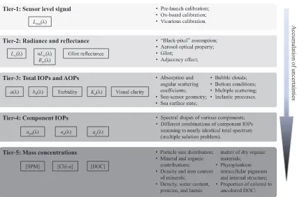
3. Theories and observations for understanding uncertainties in satellite water quality parameters
The connectivity between directly measurable light signal and de-sired water quality parameters is subject to varying degrees of un-certainties. Conceptually we can categorize satellite-derived variables into different tiers based on how many uncertainty sources are asso-ciated with each variable, which is shown inFig. 1. Variables in each tier have uncertainties accumulated from all tiers above. In other words, we expect generally least uncertainty in Tier-1 variables and most uncertainty in Tier-5 variables. Note thatFig. 1holds regardless of what approach is used to derive a satellite water quality product, either via an Inherent Optical Property (IOP)-based inversion method that explicitly derives variables belonging to the intermediate tiers, or via a reflectance band-ratio algorithm that bypasses the intermediate vari-ables. Below, we provide an overview of the uncertainties tier-by-tier.
3.1. Tier-1 to Tier-2: Deriving water-leaving radiance from sensor-level signal
Light signal detected from satellite sensorLTOA(λ), which itself is
subject to instrument calibration errors, is attributable to multiple sources which may not be relevant to water quality assessment. The ultimately desired portion of signal is carried in the upwelling light that emerges from below the water surface and has not been reflected by the bottom, which is referred to as the water-leaving radianceLw(λ). Other
portions of signal are generally unwanted for water quality assessment except for special cases such as oil spill detection and bottom type evaluation. The biggest portion comes from atmospheric molecules and aerosols which contribute∼90–99% to the total signal measured by satellite, depending on light wavelength and water brightness (IOCCG, 2010). Another source of noise arises from the direct reflection of light at the air-water interface, i.e., sun and sky glint, which can be used to detect changes of surface roughness caused by surfactants and oil slicks (Hu et al., 2009), but has nothing to do with optical properties of the water interior. Occasionally, underwater bubbles such as those in white caps and ship wakes can enhanceLw(λ) through strong backscattering and weak absorption (Zhang et al., 1998; Stramski and Tegowski, 2001; Terrill et al., 2001). Finally, water pixels located in the vicinity of brighter surfaces such as land, ice, or clouds are subject to the so-called “adjacency effect”, where light originated from brighter pixels is scat-tered into thefield of view of neighboring water pixels.
The process of subtracting atmospheric, glint, and bubble con-tributions from satellite-measuredLTOA(λ) is referred to as the“ atmo-spheric correction”(Gordon and Wang, 1994; IOCCG, 2010). A detailed discussion about atmospheric correction theory and process has been made elsewhere (e.g.,IOCCG, 2010) and is not included here. However, we note that atmospheric correction is one of the most challenging problems in satellite water quality remote sensing owing largely to the small water contribution toLTOA(λ). In addition, a particular difficulty in coastal and inland waters is the presence of absorbing aerosols such as dust, black carbon, and brown carbon. The presence of absorbing aerosols invalidates typical assumptions about the spectral shape of aerosol reflectance, which is critical to implementing atmospheric corrections that rely on spectral extrapolation of aerosol reflectance from the near-infrared (NIR) or SWIR bands to short wavelengths.
After applying atmospheric correction toLTOA(λ), the water-leaving
radianceLw(λ) can be obtained. A commonly used variable in satellite
OCR is the normalized water-leaving radiance, nLw(λ), which is
es-sentially theLw(λ) one would get if the atmosphere were absent and the sun were directly overhead. The nLw(λ) is practically equivalent to
satellite-derivedRrs(λ) with the only difference being a factor ofF0(λ).
The Lw(λ), nLw(λ), and Rrs(λ) are subject to similar number of un-certainties sources and are considered Tier-2 variables here.
3.2. Tier-2 to Tier-3: Inverting Rrs(λ) to derive total absorption and backscattering coefficients
Depending on light wavelength and water properties,Rrs(λ) can be directly proportional to, inversely proportional to, or essentially in-variant with the concentrations of optically significant substances in water, whereas IOPs likea(λ) andbb(λ) always covary positively with
their concentrations. Thus the remote detection of optically active substance generally boils down to the derivation ofa(λ) andbb(λ) from Rrs(λ). Note that this step is still implicitly carried out even when an
inverse model does not explicitly derives the IOPs. Like any inversion problem, the inversion ofRrs(λ) is underconstrained, primarily because
at most visible bands more output variables are desired than the number of given conditions. To derive bb(λ) and a(λ), assumptions must be made about the magnitudes or spectral shapes of their com-ponents, which inevitably introduce uncertainties. In this section we review these uncertainties as well as variability of Rrs(λ) caused by environmental factors as well as inelastic and multiple-scattering pro-cesses. Because of these uncertainties introduced in the derivation ofa (λ) andbb(λ), we categorize them as Tier-3 variables (Fig. 1). Influence of vertical inhomogeneity of IOPs onRrs(λ) is left out of this review for simplicity and readers are referred to studies made byZaneveld (1982), Forget et al. (2001), Stramska and Stramski (2005), Kutser et al. (2008), and Yang et al. (2013).
3.2.1. Sun-sensor geometry
In this section we discuss angular variability of the upwelling light
field below the water surface,Lu(θ′,θsun,φ,λ), which is the underwater counterpart ofLw(λ), in the angular range that is relevant to satellite
remote sensing. Standard operational satellite data processing software already addresses this variability but errors may still arise from de-parture of the actual angular shape of Lu(θ′, θsun, φ,λ) from model parameterization, especially for turbid waters with more variable par-ticulate scattering.
For pixels in a satellite swath,θ′is 0 at nadir and increases towards the edge of swath. Taking into account both cross-track and along-track angular ranges, maximum above-water view angle is 51–59° (equiva-lent to θ′= 35–40°) for SeaWiFS, MODIS, VIIRS, and SGLI, ∼35° (equivalent toθ′= 25°) for MERIS and OLCI, and 7.5–12° (equivalent toθ′= 6–9°) for OLI (Landsat-8) and MSI (Sentinel-2).
Theoretical computations made for open ocean waters suggest that the angular variation ofLu(θ′,θsun,φ,λ) is bigger for largerθsun, greater
range of θ′, higher particulate scatter, and is spectrally dependent (Morel and Gentili, 1993, 1996; Morel et al., 2002). Let us consider the worst scenario in the case of moderate resolution sensors with max-imumθ′= 40°. Using aPetzold (1972)scattering phase function (SPF), Morel and Gentili (1996)show that the variability ofLu(θ′,θsun,φ,λ)
within a 40°-cone centered around nadir is 10–75% for [Chl-a] = 0.03–3 mg m−3andθ
sun= 0–75°. Simulations made byMorel et al. (2002) using theoretical SPFs calculated for various sized spheroids suggest that this variability is about 0–100% for [Chl-a] = 0.03–10 mg m−3(sameθ
sunrange).Park and Ruddick (2005)show a much smaller variability of∼12% ([Chl-a] = 0.3–3 mg m−3,Fournier and Forand
(1994)SPFs), largely owing to the relatively smallθsun(30°) used in their simulations.
In situmeasurements of angular distribution of upwelling lightfield near surface are consistent with theoretical simulations. In a clear-water lake, measurements made by Tyler (1958) with θsun= 56.6° show that the totalLu(θ′,θsun,φ,λ) integrated across the spectral range
of 430–546 nm varies by∼40% within the 40°-cone. In subtropical Pacific, a single snapshot in the blue spectral range made byVoss et al. (2007)with [Chl-a] = 0.11 mg m−3shows a 20% variability within the 40°-cone (θsununspecified). Field measurements of bidirectional varia-bility in the angular range defined by the 40°-cone are not available at other geographical locations, although variability within larger angular ranges is reported in a few studies (Gleason et al., 2012; Antoine et al., 2013). For example, within the Snell cone (defined by the critical angle, 48.5°)Lu(θ′,θsun,φ,λ) at 406–560 nm varies by 40–50% in clear waters in the Mediterranean Sea withθsun= 7.4°, and by 50–70% in clear waters in the Beaufort Sea withθsun= 60.5° (Antoine et al., 2013).
In situobservations also suggest that variability ofLu(θ′,θsun,φ,λ) is likely to be higher in turbid waters compared with clear waters.In situ data obtained in coastal waters in the Rhone River plume in the Mediterranean Sea show that Lu(θ′, θsun, φ, λ) varies by 100–140% within the entire Snell cone, which approximately doubles the varia-bility in clear waters (Antoine et al., 2013). Similarly, the variability is ∼200% within a 45°-cone in the Chesapeake Bay, New York Bight, and Monterey Bay, which is also around twice its variability in clear waters in the Pacific Ocean and the Ligurian Sea (Gleason et al., 2012).
3.2.2. Bottom boundary conditions
The magnitude ofRrs(λ) can also be affected by light reflected from bottom of water if water is sufficiently clear and shallow. A rule of thumb to determine whether the water bottom is visible to the satellite at a given wavelength is to assess the value of thefirst optical depth, 1/ Kd (λ), above which 90% of the diffusely reflected light originates (Gordon and McCluney, 1975). If the actual water depth is deeper than
K
1/ d(λ), a negligible contribution (< 10%) from bottom reflection can be expected in satellite-derivedRrs(λ); otherwise the water should be
possible to remotely assess benthic habitats such as seagrass beds and coral reefs (e.g.,Dierssen et al., 2003; Mobley et al., 2005) and estimate bathymetry. Note that the same location can be optically shallow or deep depending on water turbidity even without a change in water depth.
3.2.3. Inelastic processes
SpectralRrs(λ) is driven by both elastic and inelastic processes but the derivation of IOPs is based only on the elastic fraction. Inelastic signals are contributed by water Raman scattering, phytoplankton fluorescence, and CDOMfluorescence. Their contributions toRrs(λ) are difficult to quantify, which depend on spectral distribution of incident solar irradiance, elastic absorption and scattering properties of the bulk water, wavelengths of excitation and emission, optical properties of the substance that produces the inelastic effect, and efficiency of the in-elastic process (∼quantum yield) (Mobley, 1994; Babin et al., 1996;
Gordon, 1999; Morel et al., 2002).
Raman scattering is characterized by a frequency shift (ranging within 3100–3700 cm−1 for water molecules) in scattered photon compared with the incident photon regardless of incident wavelength (Waters, 1995). Roughly one in ten photons scattered by water mole-cules are Raman-scattered to another wavelength (Mobley, 1994). The impact of Raman scattering on Rrs(λ) is significant in clear waters (< 10% in the blue, and∼15% at > 470 nm (Gordon, 1999)) but can be accounted for using empirical approaches (Lee et al., 2013; Westberry et al., 2013). Raman scattering is typically negligible across the visible spectrum in turbid waters because elastic scattering by suspended particles dwarfs all molecular scattering (Morel et al., 2002), and strong absorption by CDOM and suspended particles depletes photons at the excitation wavelengths.
Phytoplankton and CDOM fluorescence can significantly affect certain parts of theRrs(λ) spectrum despite the low probability of these
inelastic processes, e.g., 1–5% for chlorophyllfluorescence (Gordon, 1979; Mobley, 1994), and 0.5–1.5% for CDOMfluorescence (Mobley, 1994). This is because the emission wavelength of pure substance ex-cited by any incident light is fixed within a small spectral range, creating a concentrating effect where light energy captured across the UV–visible spectrum is focused onto a narrow band in the form of fluorescence.
Phytoplankton pigments are groups of chemically similar substances and theirfluorescence can introduce peaks toRrs(λ) spectrum. For
ex-ample, spectral features near 683–710 nm in theRrs(λ) spectrum
as-sociated with chlorophyllfluorescence have been used to detect phy-toplankton blooms in open oceans (e.g.,Neville and Gower, 1977; Hu et al., 2015) and coastal waters (e.g.,Gower et al., 2005; Hu et al., 2005). However, the contribution of chlorophyllfluorescence toRrs(λ)
can be diminished by competition from elastic particulate scattering and/or non-phytoplankton absorption at the excitation wavelengths of chlorophyllfluorescence (Gilerson et al., 2007; McKee et al., 2007b).
Thefluorescence of CDOM is spectrally broad owing to its chemical diversity. Across the visible spectrum, CDOMfluorescence contributes the most toRrs(λ) at the green portion (Hawes et al., 1992; Mobley, 1994; Huot et al., 2007), reported to be 6.5–8.5% in the Golf of Mexico (Hawes et al., 1992) and 10–20% in the CDOM-dominated Lunenburg Bay, Canada (Huot et al., 2007). Low contributions in the blue portion are associated with the shortage of solar UV irradiance which serves as the excitation source (Mobley, 1994). Lower contributions towards longer wavelengths are associated with the fast spectral decay of CDOM absorption coefficient because a photon mustfirst be absorbed before it can be emitted asfluorescence.
3.2.4. Multiple-scattering effect
Whereas the desireda(λ) andbb(λ) are single-scattering properties, in coastal and inland waters Rrs(λ) is contributed predominantly by
multiple-scattered photons. Single scattering dominates only within a top layer on the order of 1/4c(λ) thick (Jonasz and Fournier, 2011)
considering that water-leaving photons have to complete a round trip in and out of the water. As a rule of thumb, this layer is < 7% of thefirst
optical depth, calculated using the formula
= +
Kd(λ) a λ a λ( )[ ( ) 0.255 ( )]b λ (Kirk, 1984) and ω0(λ) > 0.8 for
natural suspended particles (Babin et al., 2003a; Stramski et al., 2007, 2015). Monte Carlo simulations byChami et al. (2006)show that the majority of remote-sensing signal is contributed by multiple-scattered light even for clear waters with thebb:aratio as low as∼0.03; in most turbid waters, up to∼94% ofRrs(λ) is contributed by multiple
scat-tering.
Multiple scattering introduces nonlinearity to the relationship be-tween Rrs(λ) and the ratio of bb/(a+bb), hereafter ωb(λ), but the
nonlinear relationship betweenrrs(λ) andωb(λ) appears to be robust for
a broad range of water properties, whererrs(λ) stands for the coun-terpart ofRrs(λ) just below surface. For clear and moderately turbid
waters (ωb(λ) < ∼0.2),Gordon et al. (1988)suggest that a quadratic function in the form ofrrs(λ) = g1ωb(λ) + g2ωb(λ)2can be used to
describe this nonlinear relationship, where g1and g2are coefficients
determined based on Monte Carlo simulations at various Sun angles and using an oceanic-coastal mean particulate SPF reported by Petzold (1972)(personal communications with H. R. Gordon). The regression formulas obtained byJerome et al. (1996) and Lee et al. (1999)based on similar simulations agree with that of Gordon’s within∼12% for
ωb(λ) < 0.2. Radiative transfer simulations made byMorel et al. (2002) and Park and Ruddick (2005)based on theoretical SPFs confirm the low variability in the rrs(λ)-vs-ωb(λ) relationship in this ωb(λ) range.
However, for largerωb(λ) values, theserrs(λ)-vs-ωb(λ) formulas tend to diverge, subjecting the inversion of rrs(λ) for a(λ) andbb(λ) to
sig-nificantly larger uncertainties in turbid waters.
The divergence of theserrs(λ)-vs-ωb(λ) formulas at higher turbidity might be caused by increased contribution to rrs(λ) from forward
scattered light because when multiple-scattering dominates, not only backscattered but also forward scattered light (in a single-collision sense) contributes significantly to Rrs(λ) (Park and Ruddick, 2005; Chami et al., 2006; Piskozub and McKee, 2011). It remains to be tested in future research whether there exists an optimal angular range in turbid waters, covering both backward and forward angular domains, over which the integrated volume scattering function correlates the best withrrs(λ), and how that optimal angular range changes with water
turbidity. The good proportionality found betweenrrs(λ) and total b (λ)/a(λ) in coastal waters of Great Bay (New Jersey), the Mississippi
Sound, and Lake Superior (Sydor et al., 2002) implies a great likelihood that such optimal angular ranges exist.
3.2.5. Variability of molecular and particulate scattering coefficients The total spectral backscattering coefficients of bulk waterbb(λ) is
contributed by water molecules, bbw(λ), and suspended particles, bbp(λ). The derivation ofa(λ) andbb(λ) fromRrs(λ) always necessitates
assumptions on spectral shapes ofbbp(λ), ora(λ), or their combinations.
Thebbw(λ) is considered as known but its magnitude varies with water temperature and salinity which can be important when bbw(λ)
dom-inates againstbbp(λ).
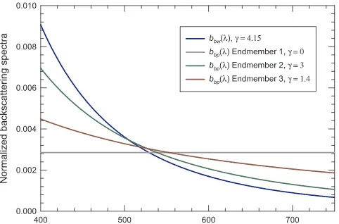
Bothbbw(λ) andbbp(λ) generally follow a power law∼λ−γ. Here we show a normalized spectrum ofbbw(λ) calculated using the formula
given byBuiteveld et al. (1994)with a depolarization ratio of 0.039 (Fig. 2). The spectral slopeγis well estimated with a small uncertainty (∼1%), and is considered invariable with temperature and salinity (Buiteveld et al., 1994; Twardowski et al., 2007; Zhang et al., 2009a), although the magnitude ofbbw(λ) does vary with these parameters.
phytoplankton cultures which tend to be dominated by algal cells with quasi-monodispersed size distribution (e.g.,Stramski et al., 2001).
Fig. 2illustrates the range of variation in spectral shapes ofbbp(λ) in
comparison withbbw(λ). Each spectrum is normalized by the integral of
the entire spectrum of 400–700 nm or 400–750 nm. For conciseness we present only endmember spectra of bbp(λ) considered realistic to
re-present natural waters. Three endmembers corresponding to extreme values ofγofbbp(λ) are shown. For suspended particles in open oceans γare found to vary from 0 to 3 (endmembers 1 and 2) (Reynolds et al., 2001; Loisel et al., 2006); for coastal particulate assemblages reported values ofγfall in a much narrower range of 0–1.4 (endmembers 1 and 3) (Babin et al., 2003a; Stramski et al., 2004b, 2007; Sydor, 2006; Snyder et al., 2008; Neukermans et al., 2014, 2016; Zheng et al., 2014; Slade and Boss, 2015). Some of the studies cited above report the spectral slope ofbp(λ) and here we consider those values equivalent to that ofbbp(λ) owing to scarcity offield-measuredbbp(λ) data. This is
acceptable since the ratio of bbp(λ)/bp(λ) is spectrally insensitive
(Stramski et al., 2004a) and we are trying to identify only endmembers of this parameter.
To understand the variability ofbbp(λ) it is helpful to examine it
from a mechanistic standpoint (Fig. 3). In a diluted medium where single-scattering dominates, bbp(λ) can be calculated as the sum of backscattering cross sectionsσbb(λ) of all suspended particles per unit
volume of water. For each individual particle,σbb(λ) can be calculated
asQbb(λ)πD2/4. TheQbbfactor depends on particle size, shape, in-ternal structure, and complex refractive index (relative to water)m(λ)
of all materials inside the particle. The real part of the index,n(main factor affecting scattering), depends mainly on density of dry mass (Aas, 1996; Woźniak and Stramski, 2004), whereas the imaginary part, n′
(main factor affecting absorption), essentially quantifies the average “darkness”of materials packed inside a particle. For organic-dominated particles including living phytoplankton and organic detritus, water content dilutes the dry mass and decreases the value ofn. In addition, inhomogeneity ofnintroduced by internal structures such as gas ve-sicles and mineral shells enhances light scattering. For example, gas vesicles can enhance the scattering efficiency of Microcystis cells by 90% to one order of magnitude (Dubelaar et al., 1987; Klemer et al., 1996; Volten et al., 1998; Matthews and Bernard, 2013). Coccolitho-phore cells are known to be effective scatterers (Balch et al., 1991) owing to their external calcite plates which has a highn-value of∼1.17 (Woźniak and Stramski, 2004). In contrast, opal (hydrated amorphous
silica, SiO2·nH2O) in diatoms has an-value of only∼1.07 (Morel and
Bricaud, 1986; Aas, 1996; Woźniak and Stramski, 2004), which is
al-most the same as that of organic particles (∼1.05,Morel and Bricaud,
1986; Bricaud et al., 1988; Aas, 1996; Stramski et al., 2001). If we ignore particle internal structure and assume that particles suspended in water are randomly oriented so that the effect of particle shape can be averaged out, we can simplify each particle as a homo-geneous sphere and the single-particle Qbb(λ) factor can be derived from the formula given byBohren and Huffman (1983, p. 383) or van de Hulst (1957, p. 35)as
∫
= ′ + ′
Q i θ n n D i θ n n D θdθ n πD λ
(λ) ( ( , , , ,λ) ( , , , ,λ))sin
( / ) ,
bb π
π
w
/2 1 2
2 (1)
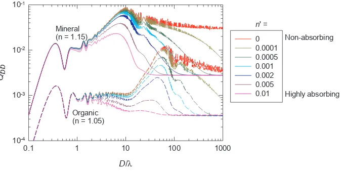
wherei1andi2are the scattered irradiances per unit incident irradiance (dimensionless irradiances) for incident light parallel and perpendicular to the scattering plane, respectively. They can be calculated usingMie (1976)theory and we used the“FASTMIE”code (https://scattport.org/ ) written by Wayne H. Slade. Results are shown inFig. 4for weakly to highly absorbing organic (n= 1.05) and mineral (n= 1.15) particles. Fig. 4provides insights to help understand the range of variability in the slope parameterγof bbp(λ). For a monodispersed particle
assem-blage, the power spectral slope γ can be calculated as Q λ D Q λ D
λ λ log[ ( , ) / ( , )]
log( / )
bb 2 bb 1
1 2 , where we chooseλ1= 400 nm andλ2= 700 nm. Among all cases inFig. 4, the steepest spectral slopeγis ∼3.8 and corresponds to non-absorbing colloids (D/λ<∼0.4). The second steepestγis∼1.7 which is found for organic particles in the size range ofD/λ= 20–60, followed by a slope of∼1.1 for mineral particles in the size range ofD/λ= 2–10. These results are consistent with the upper bound ofγ= 1.4 measured in coastal waters (Fig. 2) and indicate
that submicron sized particles are generally not important forbbpin coastal waters, whereas the steep endmember ofγ= 3 found in open
ocean waters can only be explained by a significant contribution of colloidal particles tobbp(λ).
3.3. Tier-3 to Tier-4: Attributing total absorption coefficient to components
The Tier-3 variables such asa(λ) andbb(λ) are total optical
prop-erties but remote sensing of water quality often entails partitioning them into individual components. Partitioning ofa(λ) is challenging
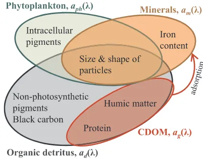
because the absorption bands of different components overlap and their spectral shapes vary. Partitioning ofbbp(λ) has not been done so far; there is not even a field methodology that separately measures its components for natural particulate assemblages. In this section, we discuss uncertainties involved in the partitioning of a(λ) into pure water,aw(λ), phytoplankton,aph(λ), suspended mineral and nonalgal organic particles,ad(λ), and CDOM,ag(λ), components, all of which are
categorized as Tier-4 variables exceptaw(Fig. 1). These components are defined on a rather arbitrary basis and largely limited by current
Fig. 2.Representative endmembers of particulate backscattering coefficientbbp(λ)
nor-malized by its integral over the entire spectrum. Endmenber 1 represents the lower bound of the power spectral slope,γ, in natural waters; 2 the upper bound ofγin open oceans; and 3 the upper bound ofγin coastal waters. Pure-water backscattering coefficientbbw(λ)
is also shown for comparison.
Fig. 3.Schematic diagram illustrating main factors that drive variations in particulate light backscattering coefficientbbp(λ) contributed by typical natural constituents such as
technical capabilities to separately measure them. Note that parti-tioning ofa(λ) into these components is physically sound because IOPs can be treated as linearly additive, i.e., we can writea(λ) =aw(λ) + aph(λ) +ad(λ) +ag(λ); this is not the case for apparent optical
prop-erties such asKd(λ), which depends not only on IOPs but also illumi-nation conditions.
3.3.1. Variability of pure water absorption coefficient
Pure water absorption coefficient aw(λ) depends on temperature
and salinity. The temperature dependency is generally small but can be significant in the vicinity of discrete bands associated with overtones and harmonics of the vibrational modes of the OeH bond (Pegau et al.,
1997; Pope and Fry, 1997; Sullivan et al., 2006; Röttgers et al., 2014). For example, local maxima of temperature-dependency were found at around 516, 606, 739, and 837 nm, whereaw(λ) changes by∼0.3, 0.5, 0.6, and 0.4% per °C, respectively (Pegau et al., 1997; Pope and Fry, 1997; Röttgers et al., 2014). The salinity dependency remains small with no more than ± 0.05% per PSU (practical salinity units) within 400–900 nm (Pegau et al., 1997; Sullivan et al., 2006; Röttgers et al., 2014).
Two endmembers of normalizedaw(λ) spectra are shown inFig. 5,
which were calculated using the formula given by Röttgers et al. (2010). Differences in these two endmembers are associated mainly with the use of two extreme temperatures (−2 and 35 °C) found in
natural seawater. Salinity effect is negligible when temperature varies within such a large range. Note thataw(λ) in the spectral region shorter than 550 nm inFig. 2a corresponds to the lowest values adopted by Röttgers et al. (2010)but there is still significant disagreement among different studies which can differ by up to > 1 order of magnitude (Pegau et al., 1997).Lee et al. (2015b)found it appealing to use even lower values within 350–550 nm to achieve a closure for remote-sen-sing reflectance measured in “clearest” subtropical gyre waters. The loweraw(λ) values was partly confirmed byMason et al. (2016)using a novel diffuse reflector that is more reflective than Spectralon (Lab-sphere Inc.). At longer wavelengths (550–800 nm), the discrepancy in estimated values ofawamong different investigators is smaller but still between 5 and 10% (Pegau et al., 1997), and the actual uncertainty in determination of each individual spectrum can be even greater ( ± 15%) (Smith and Baker, 1981).
The uncertainty in measurement of aw(λ) and its temperature/
salinity dependency deserve attention should any information con-tained in the red and NIR bands be used as a basis for invertingRrs(λ) to derive IOPs (e.g.,Shi and Wang, 2014) or water quality parameters such as [Chl-a] (e.g.,Gitelson et al., 2007). In these spectral regions the contribution of pure water to total light absorption coefficient are sig-nificant and therefore the use of accurateaw(λ) values is essential. The temperature/salinity dependency inaw(λ) can be accounted for using
formulas provided bySullivan et al. (2006)covering 400–750 nm or by
n' =
D/
0.1 1 10 100 1000
Qbb
10-4 10-3 10-2 10-1
0 0.0001 0.0005 0.001 0.002 0.005 0.01
Non-absorbing
Highly absorbing Mineral
(n = 1.15)
Organic (n = 1.05)
λ
Fig. 4.Single-particle backscattering efficiency factors cal-culated for particles suspended in water with various size (relative to wavelength) and composition (differentnandn' values) using Eq.(1)based on Mie theory. Note thatλis wavelength of light in vacuum.
Röttgers et al. (2010) and Röttgers et al. (2014) covering 400–14000 nm.
3.3.2. Variability of CDOM absorption coefficient
The endmembers ofag(λ),ad(λ), andaph(λ) are taken from a global dataset assembled byZheng and Stramski (2013)using mainly SeaWiFS Bio-optical Archive and Storage System (SeaBASS) data (Fig. 5). CDOM absorption coefficientag(λ) decays withλand the endmembers ofag(λ) were selected based on minimum and maximum values of the spectral steepness. After fitting an exponential function of λ with a single
spectral slopeSgto the measured data within 400–550 nm, we obtained the two endmembers of 0.0062 and 0.0513 nm−1, respectively (Fig. 5). Light absorption of CDOM in the visible spectral region arises mainly from proteins, humic acids, and fulvic acids (Carder et al., 1989; Wozniak et al., 2005; Loiselle et al., 2009) (Fig. 6). Terrestrial origi-nated CDOM is mainly a product of partially oxidized lignins and tan-nins (Boyle et al., 2009). Autochthonous phytoplankton-derived CDOM is believed to be produced mainly by bacteria which transform un-colored organic substance into un-colored molecules (Rochelle-Newall and Fisher, 2002b; Coble, 2007). CDOM may also be excreted by zoo-plankton (Steinberg et al., 2004). Whether phytoplankton can directly exude CDOM is still a debatable question (Rochelle-Newall and Fisher, 2002b; Castillo et al., 2010). The absorption spectral shape of auto-chthonous fulvic-acid-type CDOM produced by healthy phytoplankton is more variable than those of terrestrial originated humic and fulvic acids (Loiselle et al., 2009). The spectral slope of fulvic acids tends to be steeper than that of humic acids for both marine and terrestrial CDOM (Carder et al., 1989; Loiselle et al., 2009), followed by proteins (Wozniak et al., 2005) although there are some overlaps among these groups. Within each group the absorption efficiency may vary by more than two orders of magnitude (Wozniak et al., 2005). Many organic materials commonly found in natural waters essentially do not absorb visible light, such as aromatic amino acids, mycosporine-like amino acids, purine and pyridine compounds, and unoxidized lignins (Wozniak et al., 2005).
There is a vast body of literature on variation ofSgin the UV as-sociated with various sources and processes such as photo-bleaching and microbial consumption. For example, inland, estuarine, and coastal marine waters that receive significant amount of terrestrial-originated CDOM are found to haveflatterSgthan open oceans (Green and Blough, 1994; Del Vecchio and Subramaniam, 2004). CDOM produced by de-grading phytoplankton assumes a flatterSgin 300–500 nm compared with ambient CDOM (Zhang et al., 2009b). In contrast, photo-bleaching (Del Vecchio and Blough, 2002) and microbial activities (Nelson et al., 2004) tend to steepenSgby breaking downflat-slope CDOM into steep-slope products. These trends are observed forSgin the UV and whether they hold for the visible spectral region remains to be further in-vestigated. For example,Loiselle et al. (2009)found opposite trends with photobleaching betweenSgvalues calculated for the spectral re-gions of < 450 nm and > 500 nm.
3.3.3. Variability of nonalgal particulate absorption coefficient
The two endmembers ofad(λ) were selected in the same fashion as those forag(λ) (Fig. 5). The exponential spectral slope,Sd, of the end-members which characterizes overall spectral shape of ad(λ) ranges
from 0.0056 to 0.0193 nm−1, which is narrower than that exhibited in
ag(λ). Interestingly, the two steep-slope endmembers for ad(λ) and ag(λ) are both found in waters affected by the Amazon river plumes, whereas the flat-slope ones are both found in or near the Australian section of the Southern Ocean, which suggest possible linkages in ab-sorption properties of dissolved and particulate matter in a specific region.
Chemical composition and particle size distribution are two main factors that determine the light absorption of suspended particles comprising both organic and mineral materials. Light absorption by the organic portion of nonalgal particles arises largely from various
proteins and humic matter (Fig. 6) (Wozniak et al., 2005), similar to CDOM except that those materials are packed in particles. In addition, non-photosynthetic pigments including phaeo-pigments and car-otenoids absorb in the visible range, leading to departure ofad(λ) from
a perfect exponential function ofλ.
The most common inorganic chromophorous agent is iron (Babin and Stramski, 2004; Estapa et al., 2012) (Fig. 3a). The presence of iron uplifts the absorption spectrum ofad(λ) in the spectral region around 500 nm (Babin and Stramski, 2004; Bowers and Binding, 2006). Other minerals common to marine environments such as aluminosilicates, silicates, and carbonates generally show negligible absorption in the visible range (Babin and Stramski, 2004). Mineral absorption coeffi -cient can be enhanced by coexisting CDOM via electrochemical ad-sorption of CDOM onto the mineral surfaces (Binding et al., 2008). In addition, black carbon can be important to particulate light absorption in coastal waters near urban areas (Stramska et al., 2008) but has not been well studied.
Similar tobbp(λ),ad(λ) can be calculated as the sum of absorption cross section,σa(λ) =Qa(λ)πD2/4, of all nonalgal particles per unit volume of water, whereQa(λ) is the absorption efficiency factor and is proportional to n′(λ)D/λ(van de Hulst, 1957), independently of n. Fig. 7showsQa(λ) calculated as a function ofD/λfor particles of
dif-ferent composition using the formula fromvan de Hulst (1957). A key feature is that the increase ofQaslows down towards large values of n′(λ)D/λ owing to enhanced self-shading effect with a maximum threshold of 1 because a particle cannot absorb more light than what it physically intercepts. This feature implies thatad(λ) tends to be less wavelength-dependent for larger particles or particles composed of darker materials.
3.3.4. Variability of phytoplankton absorption coefficient
Photo-synthetic and accessory pigments dominate the light ab-sorption of phytoplankton cells. Almost all phytoplankton abab-sorption spectra share a primary peak in the blue∼440 nm and a secondary peak in the red∼670 nm. Accordingly, the two endmembers ofaph(λ)
were selected based on extreme values of the blue-to-red phytoplankton absorption band ratio, aph(440):aph(670), spanning from 1.4 to 9.1 (Fig. 5). These two endmembers define a broad range of overall spectral shape ofaph(λ) across the visible range, which is associated mainly with
cell size and intracellular pigment concentration, i.e., the degree of pigment packaging. The pigment packaging effect onaph(λ) is
essen-tially the same effect as particle size and darkness of material on the spectral slope ofad(λ). The spectrum ofaph(λ) tends to beflatter with lower blue-to-redaph(λ) band ratio for larger and more pigment-rich
cells, and vice versa.
A comparison betweenFigs. 2 and 5demonstrates that the spectral
shape ofag(λ), ad(λ), andaph(λ) vary more thanbbp(λ) does in coastal waters. As a result, the spectral shape of Rrs(λ) is dictated more by
absorption coefficients whereas the magnitude of Rrs(λ) reflects a combined effect of both absorption and backscatter.
3.4. Tier-4 to Tier-5: Deriving mass concentrations from inherent optical properties
Many applications require water quality parameters be reported in mass concentrations. The conversion from IOPs to mass concentrations is hence involved, which we categorize as Tier-5 variables (Fig. 1). Uncertainties introduced in this step arise mainly from the variability in mass-specific absorption and backscattering coefficients among various water constituents, leading to mismatches between dominant optical and mass contributors.
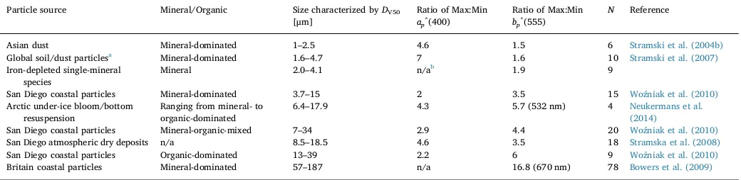
3.4.1. Variability of mass-specific optical properties of suspended particles The [SPM] is a commonly used parameter to characterize particle loading. The mass-specific IOPs of suspended particles are governed by their composition and size distribution. Many studies have reported the general variability of mass-specific IOPs resulting from the combined effect of both size and composition. Only few have examined the two effects separately. Results of these studies on mass-specific particulate absorption,ap∗(λ)≡ap(λ)/[SPM], and scattering coefficients,bp∗(λ)≡ bp(λ)/[SPM], are compared inTable 1(Stramski et al., 2004b, 2007; Bowers et al., 2009; Woźniak et al., 2010).
Table 1shows that the variability ofap∗(λ) in response to changes of particle sizeDV50is quite variable with no obvious trend. For example,
ap∗(400) can vary by as much as 7-times for a group of global soil mi-nerals with DV50ranging ∼3-folds, or as little as 2-times for another group of San Diego coastal particles withDV50ranging∼4-folds. The
lack of trend suggests thatap∗(λ) depends weakly on particle size and is primarily affected by variations in particle composition, which is also supported by limited amount of measurement data. An experiment of five pairs of particulate samples, each pair of the same composition but different size distribution, reveals some 0.7–0.9-fold of variability in ap∗(λ) per 1-fold change ofDV50ranging within 1–5μm (Stramski et al.,
2007). In contrast,ap∗(400) ranges by∼7 folds for a set of global soil mineral samples asn′(400) changes by∼6-fold (Stramski et al., 2007), and by∼4.6 folds for San Diego atmospheric dry deposits asn′(400) changes by∼4-fold (Stramska et al., 2008).
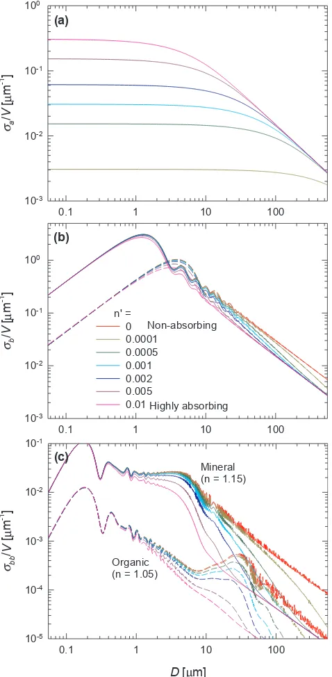
These measurement results are consistent with theoretical calcula-tions of single-particle volume-specific absorption cross-section,σa(λ)/ V, the variability of which is equivalent to that ofap∗(λ) for a hy-pothetical particulate assemblage consisting of identical particles. Calculation results at an example wavelength ofλ= 550 nm are shown
inFig. 8a, which shows thatσa(λ)/Vis fairlyflat across a broad range of Dfor each curve but changes significantly for particles with different composition (represented byn′). Thus, the use ofap∗(λ) as an avenue for estimating [SPM] depends on the uniformity of particle composition which can be quite stable, e.g., one case reported for San Diego coastal waters (Woźniak and Stramski, 2004).
In contrast to the relatively low sensitivity ofap∗(λ) to particle size variation,bp∗(λ) shows a trend of increasing variability with particle size in the size range ofDV50> 1μm (Table 1). For the smallest
parti-cles (DV50= 1–5μm)bp∗(555) varies by a factor of only 1.5–1.9 when DV50 varies by 2–3 folds. For larger particles (DV50 = 6.4–187μm)
bp∗(λ) varies by a factor of 3.5–16.8 whenDV50 varies by 2–5 folds.
Although we cannot exclude the contribution from sample-to-sample variations in organic/mineral proportions to the observed variability in bp∗(λ), it is likely that particle size plays an important role in view of theoretical considerations. Fig. 8b shows volume-specific scattering
0.1 1 10 100 1000
Qa
10-4
10-3
10-2
10-1
100
n' = Non-absorbing
Highly absorbing 0
0.0001 0.0005 0.001 0.002 0.005 0.01
n' =
D/λ
Fig. 7.Same asFig. 4but for particulate absorption efficiency factor calculated with thevan de Hulst (1957)formula.
Table 1
Variability of SPM-specific absorption and scattering coefficients of suspended particles in association with particle size and composition.DV50, median diameter of the particle volume distribution. Max, maximum value. Min, minimum value.N, number of samples.
Particle source Mineral/Organic Size characterized byDV50 [μm]
Ratio of Max:Min ap*(400)
Ratio of Max:Min bp*(555)
N Reference
Asian dust Mineral-dominated 1–2.5 4.6 1.5 6 Stramski et al. (2004b)
Global soil/dust particlesa Mineral-dominated 1.6–4.7 7 1.6 10 Stramski et al. (2007) Iron-depleted single-mineral
species
Mineral 2.0–4.1 n/ab 1.9 9
San Diego coastal particles Mineral-dominated 3.7–15 2 3.5 15 Woźniak et al. (2010) Arctic under-ice bloom/bottom
resuspension
Ranging from mineral- to organic-dominated
6.4–17.9 4.3 5.7 (532 nm) 4 Neukermans et al.
(2014)
San Diego coastal particles Mineral-organic-mixed 7–34 2.9 4.4 20 Woźniak et al. (2010)
San Diego atmospheric dry deposits n/a 8.5–18.5 4.6 3.5 18 Stramska et al. (2008)
San Diego coastal particles Organic-dominated 13–39 2.2 6 9 Woźniak et al. (2010)
Britain coastal particles Mineral-dominated 57–187 n/a 16.8 (670 nm) 78 Bowers et al. (2009)
cross-section, σb(λ)/V, calculated with Eq.(1). For both organic and mineral particles there is a maximumσb(λ)/Vlocated at around 3–5μm
for organic particles and 1–2μm for mineral particles, which explains the small variability observed for particles near these size ranges. For larger particles, the larger variability ofbp∗(λ) can be explained by the rapid changes inσb(λ)/Vwith particle size.
We also calculated the single-particle volume-specific back-scattering cross-section,σbb(λ)/V(Fig. 8c), calculated with Mie theory. Compared withσb(λ)/V(Fig. 8b), there is a broader size range within whichσbb/Vis relatively insensitive to variation of size for particles of the same composition. This explains the small variability in the mass-specific backscattering coefficient, bbp∗(λ), found in European and French Guyana coastal waters, where particle size varies within 10–140
μm butbbp∗(λ) at multiple wavelengths in the visible and NIR domain varies by only a factor of 3–4 and much of this variability could be caused by the varying degree of organic and mineral proportions (Neukermans et al., 2012). Similarly, the comparison between Figs. 8b and 8c also explains the smaller range of variability in bbp∗(532) (∼2.3 times) than that inbp∗(532) (∼5.6 times) as seen in four Arctic particulate assemblages withDV50varying within 6.4–17.9 μm and with both organic-dominated and mineral-dominated
particu-late samples (Neukermans et al., 2014).
3.4.2. Variability of chlorophyll-specific phytoplankton absorption coefficient
The [Chl-a] is another frequently used satellite water quality pro-duct. The derivation of [Chl-a] from satellite data relies mostly on the absorption signal of phytoplankton. The variability of chlorophyll-specific absorption coefficient,aph∗(λ), is spectrally minimal around the red absorption peak (∼670 nm) owing to smallest influence from ac-cessory pigments, and is higher around the blue absorption peak (∼440 nm) (e.g.,Bricaud et al., 1995; Stramski et al., 2001). Values ofaph∗(λ) determined based on data collected globally exhibit > 2 orders of magnitude variability around the blue and red absorption peaks with [Chl-a] spanning∼4 orders of magnitude (Table 2). The lowest phy-toplankton absorption per unit [Chl-a] generally decreases from open ocean, to upwelling zone, to semi-enclosed coastal waters and enclosed inland waters, with no significant difference inaph∗(λ) ranges between large-river estuaries and other“regular”coastal waters. It is common to see that a small coastal area exhibits similar or even higher degree of variability inaph∗(λ) compared with a very large oceanic region.
Much of this variability is explained by the degree of pigment-packaging effect associated with cell size and intracellular pigment concentration. For example, the average aph∗(670) of three smallest species (D= 0.7–1.4μm) in the culture dataset assembled byStramski et al. (2001)is 2-times higher than that of the two largest species (D= 12–28μm); for 11 similar sized cells (D= 4–8μm), theaph∗(670) de-cays by a factor of∼3 with intracellular chlorophyll concentration,
Ccell, ranging within 2–20 kg m−3, which can be described mathema-tically asa∗ (670)=0.0834C−
ph cell0.555 (R2 = 0.71, N = 11). Additional variability in aph∗(λ) arises from pigment composition. Presence of photoprotective pigments in high-light acclimated cells (Neukermans et al., 2014) or photosynthetic pigments in low-light acclimated cells (Bricaud et al., 1995; Babin et al., 2003a) enhances the light absorption independently from [Chl-a] thus induces a tendency of increasing aph∗(λ).
Despite the large variability ofaph∗(λ) in each dataset, the varia-bility at any given [Chl-a] rarely exceeds a factor of 5 (see references in Table 2). In addition, the calculation ofaph∗(λ) is still subject to sig-nificant measurement uncertainties for bothaph(λ) and [Chl-a].McKee et al. (2014) suggest that uncertainties of measured aph∗(λ) vary somewhere between ± 33% and ± 83%. These uncertainties imply a variability of a factor of 2, 3, and 11, respectively if we divide the upper bounds of the uncertainty ranges by the lower bounds. Therefore, the actual variability inaph∗(λ) is likely to be less than the reported ranges summarized inTable 2. Thus, the use of a [Chl-a]-dependentaph∗(λ) formula is a promising avenue to derive [Chl-a] from satellite-derived aph(λ).
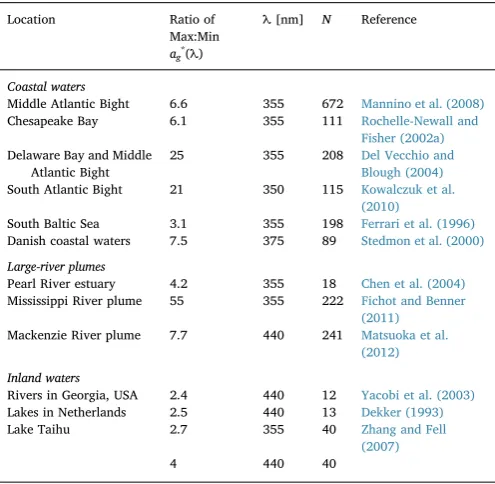
3.4.3. Variability of carbon-specific CDOM absorption coefficient Satellite data have also been used to derive the concentration of Dissolved Organic Carbon, [DOC], through the light absorption coeffi -cient of CDOM which is the colored fraction of the total DOC pool. Observed values of DOC-specific CDOM absorption coefficient,ag∗(λ) ≡ag(λ)/[DOC], vary dramatically (Table 3). An important reason is
because CDOM is a variable portion of total DOC, with the remaining portion of DOC essentially non-chromophoric and therefore not quan-tifiable with optical methods. Although the magnitude of ag∗(λ) are shown to be strongly related to the spectral slope of ag(λ) in the
0.1 1 10 100
275–295 nm region (Helms et al., 2008; Fichot and Benner, 2011, 2012), passive satellite sensors do not have the capability to make measurements in these bands. Consequently, the derivation of DOC from the light absorption coefficient is plausible only under specific conditions. For example, the quantity of uncolored DOC relative to CDOM is negligible, or uncolored DOM varies in proportion with CDOM, or the uncolored DOC is invariable, forming a stable back-ground.
A more tractable problem to pursue is the estimation of CDOM absorption coefficient normalized by its own carbon. Such studies re-quire separation of CDOM from non-chromophoric DOC and are rarely available in literature. Twardowski and Donaghay (2002) discussed reported values of carbon-normalized CDOM absorption coefficient and concluded that the difference is within 35%.Table 3shows that com-pared with regions where mixing between coastal and oceanic waters happens,ag∗(λ) is generally more constrained in inland waters where CDOM generally dominates DOC. This suggests that carbon-normalized CDOM absorption coefficient might be quite constrained, at least lo-cally.
4. Use of ocean color radiometric data for coastal pollution applications
Satellite OCR data can be used in a variety of ways to monitor and assess coastal and inland water pollution and its impacts. Representative examples of these applications are provided below, ac-companied with insights from Section3on uncertainties that can be Table 2
Variability of chlorophyll-specific absorption coefficient of phytoplankton at the blue and red absorption maxima. Samples were taken from the surface layer unless otherwise noted. Methods of [Chl-a] measurements are specified for each study.N, number of samples.
Location aph*(440) range
[m2mg−1]
aph*(670) range
[m2mg−1]
[Chl-a] range [mg m−3]
N Reference
Open oceans
Arabian Sea 0.03–0.14 0.015–0.05 0.15–2.8a 101§ Sathyendranath et al. (1999)
From Bay of Biscay to the Canary Islands 0.036–0.38 0.016–0.126 0.06–2.0c 30 Babin et al. (2003b) Subtropical gyre to Chilean upwelling zone 0.043–0.11 0.017–0.035 0.017–1.5c 66§ Bricaud et al. (2010) Patagonian shelf-break 0.018–0.173 0.009–0.046 0.1–22.3a 226‡ Ferreira et al. (2013)
A time-series station in Caribbean Sea with seasonal upwelling
0.02–0.16 0.015–0.035 0.07–8.5c 69 Lorenzoni et al. (2015)
Coastal waters
Baltic Sea 0.010–0.083 0.0077–0.049 4.35–38.7c 54 Babin et al. (2003b)
North Sea 0.003–0.10 0.0014–0.055 0.21–48.7c 88
English Channel 0.0068–0.18 0.0015–0.092 0.28–30.2c 77
Adriatic Sea 0.011–0.11 0.010–0.054 0.83–30.6c 38
Mediterranean coast 0.013–0.11 0.0045–0.045 0.09–8.5c 51
Estuaries in Queensland, Australia 0.02–0.11 0.015–0.06 0.2–8.8c 71 Blondeau-Patissier et al. (2009)
Long Island Sound ≤0.0059− 0.002–0.042 0.7–80.6a 33 Aurin et al. (2010)
Offeast coast of Malaysian Peninsular 0.004–0.23 0.001–0.027 0.11–7.7b 174 Bowers et al. (2012)
East China Sea 0.01–0.3 0.005–0.05 0.3–10a 86 Lei et al. (2012)
Hudson Bay 0.018–0.124 0.01–0.065 0.08–1.5c 54 Xi et al. (2013)
Large-river estuaries and plumes
Mississippi River Plume 0.02–0.10 0.02–0.09 0.68–12c 22 D'Sa et al. (2006)
Orinoco River plume 0.019–0.16 0.014–0.04 0.15–8.1a 73 Odriozola et al. (2007)
St. Lawrence Estuary and Gulf 0.013–0.14 0.008–0.036 0.06–16.2c 76 Roy et al. (2008)
Yellow River plume – 0.002–0.035 0.65–13.5a 62 Xing et al. (2008)
Yangtze River plume 0.017–0.16 0.008–0.055 0.1–6.1c 143‡ Wang et al. (2014)
Inland lakes
Lake Erie, USA 0.013–0.51 0.007–0.157 0.3–70b 90 Binding et al. (2008)
Lake Taihu, China 0.016–0.18 0.006–0.057 2.1–104b 57 Le et al. (2009)
Mixed water types
St. Lawrence Estuary and Gulf; Pacific and Atlantic Oceans; Mediterranean Sea
0.01–0.18 0.005–0.06 0.02–25a,b,c 815§ Bricaud et al. (1995)
aChl-aand pheopigments measured with
fluorometric methods. bChl-aand pheopigments measured with spectrophotometric methods. cTotal Chl-ameasured with the HPLC method.
§Sampling depth varies within the euphotic zone.
‡Sampling at surface and the Chl maxima layer.
Table 3
Variability of DOC-specific absorption coefficient of CDOM. Max, maximum value. Min, minimum value.N, number of samples.
Location Ratio of Max:Min ag*(λ)
λ[nm] N Reference
Coastal waters
Middle Atlantic Bight 6.6 355 672 Mannino et al. (2008) Chesapeake Bay 6.1 355 111 Rochelle-Newall and
Fisher (2002a) Delaware Bay and Middle
Atlantic Bight
25 355 208 Del Vecchio and Blough (2004) South Atlantic Bight 21 350 115 Kowalczuk et al.
(2010)
South Baltic Sea 3.1 355 198 Ferrari et al. (1996) Danish coastal waters 7.5 375 89 Stedmon et al. (2000)
Large-river plumes
Pearl River estuary 4.2 355 18 Chen et al. (2004) Mississippi River plume 55 355 222 Fichot and Benner
(2011) Mackenzie River plume 7.7 440 241 Matsuoka et al.
(2012)
Inland waters
Rivers in Georgia, USA 2.4 440 12 Yacobi et al. (2003) Lakes in Netherlands 2.5 440 13 Dekker (1993)
Lake Taihu 2.7 355 40 Zhang and Fell
(2007)
![Fig. 11. Regression relationships between [SPM] and in situ measuredremote-sensing reflectance](https://thumb-ap.123doks.com/thumbv2/123dok/2432880.1645506/16.595.39.350.529.737/fig-regression-relationships-spm-situ-measuredremote-sensing-reectance.webp)
