www.elsevier.com/locate/dsw
Group technology approach to the open shop scheduling
problem with batch setup times
V.A. Strusevich
∗School of Computing and Mathematical Sciences, University of Greenwich, 30 Park Row, London SE10 9LS, UK
Received 1 November 1998; received in revised form 1 December 1999
Abstract
This paper studies the problem of scheduling jobs in a two-machine open shop to minimize the makespan. Jobs are grouped into batches and are processed without preemption. A batch setup time on each machine is required before the rst job is processed, and when a machine switches from processing a job in some batch to a job of another batch. For this NP-hard problem, we propose a linear-time heuristic algorithm that creates a group technology schedule, in which no batch is split into sub-batches. We demonstrate that our heuristic is a 5
4-approximation algorithm. Moreover, we show that no group technology algorithm can guarantee a worst-case performance ratio less than 5
4. c2000 Elsevier Science B.V. All rights reserved.
Keywords:Open shop; Batching; Group technology; Approximation
1. Introduction
In this paper, we consider the two-machine open shop scheduling problem with batch setup times. This problem is a modication of the conventional version of the two-machine open shop problem without batching and setups, which is one of the classical multi-stage models in scheduling theory.
In the classical case, we are given a setN={1;2; : : : ; n}of jobs to be processed on two machines, AandB, without preemption. The processing times of each job on each machine are known. Neither of the machines can process more than one job at a time. For every job, the processing route, i.e., the order in which the job passes the machines, is not given in advance and has to be chosen, dierent jobs being allowed to follow
∗Corresponding author. Fax: +44-181-3318665.
E-mail address: [email protected] (V.A. Strusevich)
dierent routes. Thus, a job can be assigned rst to machine A and then to machineB, while for another job the opposite route can be selected. The objective is to nd a schedule that minimizes the makespan Cmax,
which is the completion time of all jobs on both machines. Following a standard classication scheme [5], this problem is denoted byO2kCmax.
A more general situation to be found in certain manufacturing environments involves a setup performed on a machine before it can start the processing of a job. In other words, performing a job on a machine consists of two phases: the setupphase, which is followed by the processingphase. In this paper, we assume that the setup times are sequence-independent, i.e., they depend only on the machine and on the job that follows the setup. For the two-machine open shop, we assume that the setup for any job on a machine can be performed simultaneously with any activity on the other machine, including the setup for the same job. However, as in the classical case, the processing of a job on both machines at the same time is forbidden. We denote the resulting problem by O2|setup|Cmax, provided that the makespan is chosen as the objective.
The open shop model with batch setup times, which is the main object of study in this paper, is similar to problem O2|setup|Cmax. Here, however, the jobs are known to be partitioned into groups, calledbatches. No
setup is incurred between jobs of the same batch. On the other hand, a setup on each machine is required before the rst job assigned to the machine is processed, and when a machine switches from processing a job in some batch to a job of another batch. This problem is denoted by O2|batch setup|Cmax.
Generally speaking, in the problems with batch setup times the given batches of jobs can be split into smaller groups, called sub-batches. The rst job of each sub-batch needs a setup. In this paper, we consider a restricted class of scheduling algorithms for problem O2|batchsetup|Cmax. Often implemented in practice
and known as group technology methods, the algorithms of this class schedule each batch as a whole block of jobs without splitting it into sub-batches. For various scheduling problems with batch setup times, group technology algorithms cannot deliver a global optimal solution, but they appear to be able to create schedules reasonably close to optimal ones.
Closely related to the model discussed in this paper are scheduling problems based on a dierent machine environment, known asow shop. In the two-machine case, the dierence between the open shop and the ow shop is that, for the ow shop, each job is rst processed on machineAand then on machineB, while for the open shop determining the job processing routes is part of the scheduling decision-making. Similarly to its open shop counterpart, the two-machine ow shop problems to minimize the makespan with no setups, with job setup times and with batch setup times are denoted byF2kCmax,F2|setup|Cmax, andF2|batchsetup|Cmax,
respectively.
We recall main complexity results on relevant scheduling problems. Problems O2||Cmax andO2|setup|Cmax
are solvable in O(n) time due to Gonzalez and Sahni [2] and Strusevich [6], respectively. Both problems
F2||Cmax andF2|setup|Cmax are solvable in O(nlogn) time due to Johnson [3] and Yoshida and Hitomi [7],
respectively. On the other hand, both problems F2|batchsetup|Cmax and O2|batch setup|Cmax are NP-hard
as proved by Kleinau [4]. The latter facts motivate design and analysis of approximation algorithms for the problems with batch setup times.
For a scheduling problem to minimize the makespan, a heuristic algorithm is called a -approximation
algorithm, if for any instance of the problem it creates a schedule with the makespan that is at most times the optimum value. If is as small as possible, then is the worst-case performance ratio of the heuristic. Two O(nlogn) time heuristic algorithms for problemF2|batch setup|Cmax are given by Chen et al. [1]. One
of these algorithms is a 3
2-approximation group technology algorithm. Moreover, it is shown that no group
technology algorithm can guarantee a worst-case performance ratio smaller than 32. Further, by allowing each batch to be split into at most two sub-batches, a second heuristic is developed for which a reduced worst-case performance ratio of 43 is obtained.
The purpose of this paper is to analyze the group technology approach to solving problemO2|batchsetup|Cmax.
We demonstrate that no group technology algorithm can guarantee a worst-case performance ratio smaller than
5
4, and present a 5
This paper is organized as follows. Section 2 provides preliminary results and discusses schedules found by reducing problem O2|batchsetup|Cmax to the problem with job setup times. In Section 3 we consider special
ow shop schedules for processing jobs of a specic batch. Our main heuristic and its analysis are presented in Section 4. The aspects of tightness of the obtained ratio bounds are outlined in Section 5.
2. Preliminaries
We start with a formal description of problem O2|batchsetup|Cmax, introduce some notation and analyze
a schedule found by reducing the original problem to problem O2|setup|Cmax.
In problem O2|batchsetup|Cmax, we are given the set N={1;2; : : : ; n} of jobs. Each job j∈N must be
processed on machines A and B; the processing times areaj andbj, respectively. SetN is partitioned into batches N1; : : : ; N. Batch setup times of batch N for 166 on machines A and B are equal to s
A andsB time units, respectively. For an arbitrary scheduleS, the makespan, or the length, of the schedule is denoted by Cmax(S). An optimal schedule with the smallest possible makespan is denoted by S∗.
Given a scheduling problem, in order to specify a schedule for all of some of the jobs we have to provide information on the starting and/or completion times of every job on each machine. Since the open shop with batch setup times is a suciently complicated model, to avoid confusion we need a tool for formal description of schedules.
In what follows, a scheduleS is specied by a pair of strings of the form (L;H1;H2;: : :;HhL), wherehL¿1.
Here L∈ {A; B} is the name of a machine, and an item Hj of the string is of the form [Rj(L); j(Nj)], which indicates that machine L, beginning at time Rj(L), processes the jobs of setNj according to the permutation
j(Nj) and does not become idle until it has performed all these jobs. The setup times are incurred whenever the machine switches from a job in one batch to a job in another batch. If the rst job in the sequence j(Nj) is the rst job in its batch, then Rj(L) corresponds to the starting time of the batch setup; otherwise Rj(L) corresponds to the starting time of the processing of the rst job in j(Nj). There is no idle time between the completion of a batch setup and the processing of the rst job in the batch. A similar representation of schedules in terms of a pair of strings is used in [6].
For a non-empty subset Q⊆, denote
a(Q) =X
For any schedule S for problem O2|batchsetup|Cmax, the makespan cannot be smaller than the workload
of a machine. Besides, the amount of time needed to complete a job j from a batch N is either at least
s
A+aj+bj, if the job is given the processing route (A; B), or at least sB+aj+bj, if the job is given the opposite route (B; A). Thus, a lower bound on the makespan can be written as
Cmax(S)¿max{TA; TB;max{min{sA; sB}+aj+bj|j∈N; 166}}: (1)
Recall that our goal is to design a group technology algorithm for problemO2|batchsetup|Cmaxthat provides
Given an instance of problemO2|batchsetup|Cmax withbatches, transform it into an instance of problem O2|batchsetup|Cmax with composite jobs J1; J2; : : : ; J. This is done by replacing each batch N, 166, by an articial job J assuming that the processing times of J on machines A andB are given by
=a(N); =b(N);
respectively, and the job setup times are given by
s; A=sA; s; B=sB:
Using the algorithm given in [6] applied to the jobs J1; J2; : : : ; J, we may nd a schedule S for problem
O2|setup|Cmax such that
Cmax( S) = max
(
X
=1
(s; A+); X
=1
(s; B+); max{min{s; A; s; B}++|166} )
:
By the inverse substitution of each composite job J by an arbitrary sequence of the jobs of batch N, schedule S can be transformed into a schedule S0 for the original problem O2|batchsetup|Cmax such that
Cmax(S0) = max{TA; TB;max{min{sA; sB}+a(N) +b(N)|166}}:
Obviously, S0 is a group technology schedule, i.e., each batch is processed as a block. Moreover, since in
schedule S no job is processed by both machines at a time, we derive that there is no batch overlapping in schedule S0. Notice that nding schedule S0 requires O(n) time.
We need to consider the case that
Cmax(S0)¿max{TA; TB};
since otherwise schedule S0 is optimal due to (1).
Without loss of generality, assume that the batches and the machines are numbered and named in such a way that
Cmax(S0) =sA1+a(N1) +b(N1): (2)
We will refer to batch N1 as the long batch. Again, we only have to consider the case that the long batch
contains more than one job; otherwise S0 is optimal.
Note that (2) implies that
s1A+a(N1)¿ TB−(s1B+b(N1)); b(N1)¿ TA−(s1A+a(N1)) (3)
and
s1A6s1B: (4)
Due to (2), we observe that in order to reduce the makespan we must allow the processing of the long batch on one machine overlap with its processing on the other machine. Some useful schedules of this type are discussed in the following section.
3. Flow shop schedules for the long batch
We now present an approach to nding ow shop schedules for the jobs in the long batch in linear time. The approach is based on the Gonzalez–Sahni algorithm for problem O2||Cmax or its extension for problem O2|setup|Cmax (see [2,6]).
For problem O2|batchsetup|Cmax, temporarily disregard all batches other than the long batch N1. Our
current purpose is to nd a schedule in which the jobs of N1 are processed as in a ow shop, i.e., either they
Let (Q) denote an arbitrary permutation of the jobs of a non-empty set Q⊆N, while (∅) stands for a dummy permutation. Split batch N1 into two subsets one of which may be empty:
NA1={j∈N1|aj6bj}; NB1=N1\NA1:
Select the jobsl∈NA1 such thatbl¿max{aj|j∈NA1}, and r∈NB1 such thatar¿max{bj|j∈NB1}. If either of the sets NA1 or NB1 is empty, then assume either {l}=∅ or {r}=∅, respectively. Form two permutations
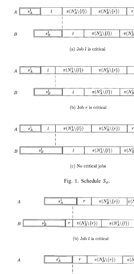
’(N1) = (l; (NA1\ {l}); (NB1\ {r}); r) and (N1) = (r; (NB1\ {r}); (NA1\ {l}); l).
Following [2] (see also [6]), we may dene a ow shop schedule S’ for processing the jobs of batch N1 that is specied by the pair of strings
(A; [0; ’(N1)]);
(B; [max{s1
A+al−s1B; s1A+a(N1)−(s1B+b(N1\ {r}));0}; ’(N1)]):
In this schedule, each job is completed on machineA before it starts on machine B. If a schedule contains a job that starts on one of the machines exactly when it is completed on the other machine, the job is called critical.
Lemma 1. If schedule S’ has a critical job; then either jobl is critical and the inequalities
s1A+al¿sB1
and
a(N1\ {l})6b(N1\ {r}) (5)
hold; or job r is critical and(5) does not hold.
We skip the Proof of Lemma 1, since it is straightforward to adapt the proofs of similar statements given in [1,2,6]. Fig. 1 shows possible shapes of schedule S’. In this and subsequent gures, a double-framed box represents a setup.
Similarly, dene a ow shop schedule S that is specied by the pair of strings
(A; [max{s1
B+br−s1A; s1B+b(N1)−(s1A+a(N1\ {l})}; (N1)]); (B; [0; (N1)]):
In this schedule, all jobs are rst processed on machine B and then on machine A. Observe that due to (4) schedule S always contains a critical job. Moreover, if (5) holds then job l is critical; otherwise job r
is critical (see Fig. 2).
We use schedules S’ andS and their properties in the subsequent algorithm in its analysis.
4. Main algorithm
We now present a linear-time group technology algorithm that nds a schedule SH for problemO2|batch
setup|Cmax, such that Cmax(SH)654Cmax(S∗). The algorithm starts with nding schedule S0 in which each
batch is treated as an individual articial job. If the length of schedule S0 is determined by the time needed
to setup and process the long batch, the algorithm nds a number of schedules and accepts the best found schedule as a heuristic solution.
In all schedules created by the algorithm, the batches dierent from the long batch are kept as a block. DeneN0=N2∪N3∪ · · · ∪N. Let (N0) denote a permutation of jobs obtained by sorting the jobs in each
Fig. 1. ScheduleS’.
Fig. 2. ScheduleS .
In some of the schedules created by the algorithm, the jobs of the long batch are sequenced as in schedules
S’ orS , described in the previous section. For a job j∈N1, we write’(N1\ {j}) to denote the permutation obtained from ’(N1) by deleting job j. The notation (N1\ {j}) is used analogously.
Algorithm H.
1. Find scheduleS0. Identify the long batch. If necessary, renumber the batches so that the long batch is batch N1. If necessary, rename the machines so that (4) holds. If either C
max(S0)¡ s1A+a(N1) +b(N1) or batch
2. If inequality (5) holds, then nd the schedules that are specied by the pairs of strings I–V given below.
3. If inequality (5) does not hold, nd the schedules that are specied by the pairs of strings VI–XII given below. Go to Step 4.
It is easily verify that Algorithm H requires O(n) time. If the conditions of Step 1 hold, then, as shown in Section 2, schedule S0 is optimal. In the lemmas below, we analyze the worst-case performance of Algorithm
H. Recall that the algorithm enters either Step 2 or Step 3 provided that relations (3) and (4) hold.
Theorem 1. Let SH be the best schedule found in Step 2 of Algorithm H. Then the following bound
Cmax(SH)654Cmax(S∗) (6)
holds.
Proof. First, observe that in Step 2 of Algorithm H inequality (5) holds. Due to Lemma 1, this implies that if either schedule S’ or scheduleS has a critical job, then this job is job l.
Let S1 be the schedule specied by the pair of strings I. First of all, observe, that the jobs of set N0 do
not overlap due to (3), while each job of batch N1 starts on machine B no earlier than in schedule S’. If either machine A terminates schedule S1 or there is no idle time on machine B, then Cmax(S1) =
max{TA; TB} and S1 is optimal. Therefore, assume that machine B terminates this schedule and that there
is idle time onB. This implies that the jobs of the long batch N1 are processed in scheduleS
1 exactly as in impossible due to (1). Therefore, it follows from (4) and (8) that
not overlap, while job lstarts on machine B after it is nished on A.
If machine B terminates the schedule then Cmax(S2) = max{sA1+al+bl; TB} and this schedule is optimal. Thus, assume that machineAterminates schedule S2 and there is idle time onA, since otherwise S2 is optimal.
We obtain
Cmax(S2) =TB−bl+TA−s1A−al:
Thus, ifs1
A+al+bl¿34Cmax(S∗), thenCmax(S2)654Cmax(S∗). Therefore, in what follows, it is assumed that
s1A+al+bl¡34Cmax(S∗): (12)
Moreover, we only need to consider the case when
b(N1\ {l})¿1
2Cmax(S ∗
); (13)
Let S3 be the schedule specied by the pair of strings III. Observe that the jobs of set N0 do not overlap
due to (3), while each job of batch N1 starts on machineA no earlier than in schedule S . Again, we only
have to consider the case when machine A terminates this schedule and there is idle time on that machine, otherwise S3 is optimal. By moving job l to the rst position in batch N1 on machine A, transform this
schedule into a new schedule S4 that is specied by the pair of strings IV. Observe that in this schedule each
job of set N1\ {l} starts on machine Ano earlier than in schedule S
3, while job lstarts on Bno earlier than
this job is completed on A. This also implies that the jobs of set N0 do not overlap.
If either machine A terminates this schedule or there is no idle time on machine B, then Cmax(S4) =
max{TA; TB} and S4 is optimal. Therefore, assume that machine B terminates this schedule and there is idle
time on B.
By moving joblto the rst position in batchN1 on machineB, transform scheduleS
4 into a new schedule S5 that is specied by the pair of strings V. Observe that in this schedule there is no job overlap.
If either machine B terminates this schedule or there is no idle time on A, then Cmax(S5) = max{TA; TB} and S5 is optimal. Suppose that machine A terminates this schedule and there is idle time on A, so that
Cmax(S5) =sB1+b(N1) +a(N1\ {l}):
It follows from (14) that Cmax(S5)654Cmax(S∗).
Thus, we have proved that if SH is the best of the schedules dened by the pairs of strings I–V, then the required bound (6) holds.
We now analyze the schedules found in Step 3 of Algorithm H.
Theorem 2. Let SH be the best schedule found in Step 3 of Algorithm H. Then the bound (6) holds.
Proof. First, observe that in Step 3 of Algorithm H inequality (5) does not hold. Due to Lemma 1, this implies that if either schedule S’ or schedule S has a critical job, this is job r.
Let S6 be the schedule specied by the pair of strings VI. Due to (3), the jobs of set N0 do not overlap.
Besides, each job of batch N1 starts on machine B no earlier than in schedule S
’.
If either machine A terminates schedule S6 or there is no idle time on machine B, then Cmax(S6) =
max{TA; TB} and S6 is optimal. Therefore, assume that machine B terminates this schedule and there is
since r∈N1
not overlap, while job r starts on machine B after it is nished onA.
Assume that machine A terminates schedule S7, and there is idle time on A; since otherwise S7 is optimal.
Thus, we obtain
Cmax(S7) =TB−br+TA−s1A−ar:
Thus, ifs1A+ar+br¿34Cmax(S∗), then Cmax(S7)654Cmax(S∗). Therefore, in what follows, it is assumed that
s1A+ar+br¡34Cmax(S∗); (19)
Moreover, we only need to consider the case when
a(N1\ {r})¿21Cmax(S∗); (20)
since otherwise Cmax(S6)654Cmax(S∗) due to (15) and (19).
We split our consideration into two cases, depending on the size of the batch setup time s1
B.
Let S8 be the schedule specied by the pair of strings VIII. Due to (20) and (21) we have
X
=2
(sA+a(N)) +s1A+ar612Cmax(S∗)¡ s1B;
therefore, in schedule S8 job r starts processing on B after it is completed on A. Observe that machine B always terminates schedule S8, so that Cmax(S8) = max{TB; TA+P=2(sB +b(N)) +b(N1\ {r})} and
Cmax(S8)654Cmax(S∗) due to (22).
Case2: Suppose now that (21) does not hold.
Case2.1: Assume that the following inequality
Consider a new schedule S9 that is specied by the pair of strings IX. Observe that in this schedule the
jobs of set N1\ {r} and those of set N0 do not overlap, while job r starts on A no earlier than this job is
completed on B.
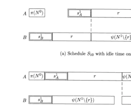
Fig. 3. SchedulesS10 andS11.
If machine A terminates scheduleS9 thenCmax(S9) = max{TA; s1B+br+ar}, so that Cmax(S9)654Cmax(S∗)
due to (19) and because (21) does not hold.
Case2.2: We now assume that the inequality
s1B+br612Cmax(S∗) (24)
holds.
Consider schedule S10 that is specied by the pair of strings X. We only have to look at the case when
machine A terminates schedule S10 and there is idle time x(S10) on A (see Fig. 3(a)). Due to (24) we have 1
2Cmax(S
∗ )¿s1
B+br¿x(S10). This implies
x(S10)¿14Cmax(S∗) +br: (25)
Transform schedule S10 into a new schedule S11 in the following way:
1. Temporarily remove job r and the sequence of jobs (N0) on machineB.
2. Start the setup for batch N1 on machine A immediately after the block of jobs (N0) is completed, and
start the processing of job r on that machine immediately after the setup. 3. Reduce the starting times of all jobs of set N1\ {r} on machineB by b
r. 4. Reduce the starting times of all jobs of set N1\ {r} on machineA by min{b
r; x(S10)}.
5. Make job r the last job in batch N1 on machines B and start the processing of job r as early as possible,
i.e., either when job r is completed on A or when the last job in the sequence (N1\ {r}) is completed
on B.
6. Start the sequence (N0) on B as soon as job r is completed on that machine.
As a result, we obtain schedule S11 that is specied by the pair of strings XI. Observe that the above
transformations reduce the idle time on A by at least br compared with that in schedule S10. Therefore, if
machine A terminates schedule S11, then due to (25) we have Cmax(S11)6TA+ 14Cmax(S∗)654Cmax(S∗). If
machine B terminates schedule S11 then we only have to consider the case when there is idle time on B;
otherwise S11 is optimal (see Fig. 3(b)).
Letx(S11) =P=2(sA+a(N)) +sA1+ar−(sB1+b(N1\ {r})) denote the idle time on machineBin schedule
S11.
If Cmax(S11)¿54Cmax(S∗) then x(S11)¿14Cmax(S∗). It follows from (20) that
1 2Cmax(S
∗ )¿
X
=2
(sA+a(N)) +s1A+ar¿ s1B+b(N1\ {r}) +14Cmax(S
implying
s1B+b(N1\ {r})¡14Cmax(S∗): (26)
Consider a new schedule S12 that is specied by the pair of strings XII. We only have to look at the case
when machine B terminates schedule S12 and there is idle time on B. We obtain Cmax(S12) =s1A+a(N1) +
b(N1\ {r}), and by (26) we derive C
max(S12)654Cmax(S∗).
Thus, we have proved that if schedule SH is the best of all schedules found in Step 4 then the desired bound (6) holds.
5. Tightness
It follows from Theorems 1 and 2 that Algorithm H provides a worst-case ratio bound of 54. In this section we demonstrate that this bound cannot be improved by any group technology algorithm.
To see that 54 is a tight bound, consider the following instance of problem O2|batchsetup|Cmax. There are
two batches each consisting of two identical jobs: N1={1;2}; N2={3;4}. All batch setup times are zero,
while processing times are as follows:
a1=a2= 2; b1=b2= 1; a3=a4= 0; b3=b4= 1:
It is easy to see that there exists an optimal schedule with the makespan of 4 in which, e.g., machine
A processes the jobs in the sequence (1,2) and machine B in the sequence (3,2,1,4). On the other hand, Algorithm H outputs a schedule with the makespan of 5.
Moreover, considering the same example it is easy to verify that there is no schedule in which a batch is not split into sub-batches and which has a makespan smaller than 5. Thus, Algorithm H is a best possible heuristic algorithm for problem O2|batchsetup|Cmax, which employs the group technology approach. Notice
that for the ow shop counterpart of out model, i.e., problem F2|batchsetup|Cmax, a best-possible group
technology algorithm gives a ratio of 3
2 (see [1]).
Possible next steps in studying problem O2|batch setup|Cmax may include the development of an algorithm
that will allow batch splitting, e.g., at least once. It is still an open question whether the problem admits a fully polynomial approximation scheme, or at least a polynomial approximation scheme.
References
[1] B. Chen, C.N. Potts, V.A. Strusevich, Approximation algorithms for two-machine ow shop scheduling with batch setup times, Math. Programming B 82 (1998) 255–271.
[2] T. Gonzalez, S. Sahni, Open shop scheduling to minimize nish time, J. Assoc. Comput. Mach. 23 (1976) 665–679.
[3] S.M. Johnson, Optimal two- and three-stage production schedules with setup times included, Naval Res. Log. Quart. 1 (1954) 61–68. [4] U. Kleinau, Two-machine shop scheduling problems with batch processing, Math. Comput. Modelling 17 (1993) 55–66.
[5] E.L. Lawler, J.K. Lenstra, A.H.G. Rinnooy Kan, D.B. Shmoys, Sequencing and scheduling: algorithms and complexity, in: S.C. Graves, A.H.G. Rinnooy Kan, P. Zipkin (Eds.), Handbooks in Operations Research and Management Science, Vol. 4, Logistics of Production and Inventory, North-Holland, Amsterdam, 1993, pp. 445 –522.
[6] V.A. Strusevich, Two machine open shop scheduling problem with setup, processing and removal times separated, Comput. Oper. Res. 20 (1993) 597–611.