Full Terms & Conditions of access and use can be found at
http://www.tandfonline.com/action/journalInformation?journalCode=ubes20
Download by: [Universitas Maritim Raja Ali Haji] Date: 12 January 2016, At: 01:07
Journal of Business & Economic Statistics
ISSN: 0735-0015 (Print) 1537-2707 (Online) Journal homepage: http://www.tandfonline.com/loi/ubes20
Nonmarket Household Time and the Cost of
Children
Christos Koulovatianos, Carsten Schrder & Ulrich Schmidt
To cite this article: Christos Koulovatianos, Carsten Schrder & Ulrich Schmidt (2009)
Nonmarket Household Time and the Cost of Children, Journal of Business & Economic Statistics, 27:1, 42-51, DOI: 10.1198/jbes.2009.0004
To link to this article: http://dx.doi.org/10.1198/jbes.2009.0004
View supplementary material
Published online: 01 Jan 2012.
Submit your article to this journal
Article views: 80
Nonmarket Household Time and the
Cost of Children
Christos K
OULOVATIANOSDepartment of Economics, University of Exeter, Exeter, EX4 4PU, United Kingdom (c.koulovatianos@exeter.ac.uk)
Carsten S
CHRO¨ DERDepartment of Economics, University of Kiel, Kiel, D-24098, Germany (carsten.schroeder@bwl.uni-kiel.de)
Ulrich S
CHMIDTDepartment of Economics, University of Kiel, Kiel, D-24098, Germany and Kiel Institute for the World Economy, Kiel, D-24105, Germany (uschmidt@bwl.uni-kiel.de)
Raising children demands a considerable amount of parental time, obliging working parents either to reduce their leisure time further or to buy childcare services in the market. Parents may face additional opportunity costs upon deciding to participate in the labor market, but these are difficult to measure. Using a survey instrument in Belgium and Germany, we estimate the income compensation needed to maintain family well-being when adults work versus when they do not enter the labor market. In both countries we find that full-time working parents face extra child costs and require higher labor market participation compensation compared with childless adults.
KEY WORDS: Child costs; Equivalent income; Household well-being; Parental unemployment trap; Reservation wage; Survey method.
1. INTRODUCTION
In a literature survey about how children affect the economic behavior of households, Browning (1992) noted:
Every aspect of household economic behavior is significantly correlated with the presence of children in the household. [. . .] children [. . .] do play a central
role in understanding all facets of household economic behavior. (pp. 1470– 1471)
A particular feature of households with children is that chil-dren must be raised by the adults in the household. Childcare requires the investment of time, effort, and other resources on the part of adult household members. The constraints faced by adults in this regard are affected by the labor market partic-ipation status of the adult household members: Working adults have less nonmarket time available for childcare and other household production activities than do nonworking adults.
We designed a survey instrument to estimate the tradeoff between nonmarket time and household income. This tradeoff is given by the income compensation for a reduction in non-market time required to keep family well-being constant. Empirically, we investigated whether the time/money tradeoff is higher in households with children versus those without children. Furthermore, we estimated child costs for households with working versus nonworking adults. Such estimates help in evaluating whether transfers to reduce child poverty are equi-table across different household types. Examining whether children affect labor market participation compensation ena-bles us to evaluate whether tax allowance policies that reward working parents create sufficient work incentives to move parents out of an unemployment/poverty trap (for example, see Brewer 2001, who discusses related policies in the United States and the United Kingdom).
Econometric approaches such as those suggested in Apps and Rees (2001) specify demand systems to estimate child costs in different household types from consumption and time–
use data. Various factors make this approach challenging. No existing database drawn from the same sample of households contains information about both time–use and consumption (Gronau and Hamermesh 2006, p. 3). Even if such a database existed, its informational content would be limited. For example, the variable ‘‘wage’’ can be observed only for the subsample of working people, making—effectively—a sample selection correction necessary (Wooldridge 2002, p. 552). Other information is not collected at all, such as the extent to which household members share goods within the household; the quantity/quality of domestic production; and, not least, ‘‘who gets what’’ (Browning 1992, p. 1470). As a result, to infer prices of domestic goods, including the value of time that adults devote to child-related activities, estimated demand systems depend critically upon (a priori untestable) exogeneity assumptions, assumptions on within-household sharing rules and functional forms of household production processes, as well as identification restrictions (for example, see Donaldson and Pendakur 2004, 2006 for references concerning restric-tions such as ‘‘equivalence-scale exactness’’ used to identify household cost functions, and generalizations they suggest).
Our approach does not rely upon the specification of a theo-retical model and thus avoids the need to make modeling assumptions that are a priori untestable. Our survey method requires respondents to perform a set of evaluation tasks that are directly related to the estimation of child costs in different household types. Similar to Koulovatianos, Schro¨der, and Schmidt (2005), our approach relies on the idea that respondents, based on their daily experiences and choices, are capable of providing reliable assessments when asked the following
42
2009 American Statistical Association Journal of Business & Economic Statistics January 2009, Vol. 27, No. 1 DOI 10.1198/jbes.2009.0004
types of questions: Which family income level can make a household with one working and one nonworking adult with two children achieve the same well-being as a household with a nonworking, single, childless adult and a monthly family income of $1,000, in your opinion? What income would one need if, instead, both adults were nonworking? If both adults were working? The answers we obtain are equivalent incomes (i.e., disposable family incomes that make the well-being of households with different demographic composition and labor market participation status equal). So, the time/money tradeoff is captured by the difference between equivalent incomes of two household types that differ only with respect to the nonmarket time endowment (NMTE) of adult household members.
We conducted this survey in two countries (Belgium and Germany), focusing on two types of reductions in NMTE. Starting from a household in which all adult members are nonworking, we distinguished (1) a nonrestrictive reduction in NMTE that leads to a ‘‘traditional’’ household with one working and one nonworking adult, and (2) a restrictive reduction in NMTE that leads to a situation in which all adults in the household work full time. We found that the time/money tradeoff corresponding to nonrestrictive reductions in NMTE is typically unaffected by the presence of children in the house-hold. On the contrary, in both countries, it was always the case that, in response to a restrictive reduction in NMTE, the time/ money tradeoff increased whenever children were present.
As a robustness check, we used regression analysis to esti-mate child costs relative to an adult, after controlling for economies of household size and also for several personal characteristics of the survey’s respondents. Consistent with our results just mentioned, child cost estimates are higher in time-constrained families when compared with households in which at least one adult is nonworking. These findings suggest that parents may face additional opportunity costs upon deciding to start working full time, except in one important case: when one of the two nonworking parents decides to go to work. Accord-ingly, income tax allowance policies that aim to increase work incentives need to favor working parents.
Our results also have broader implications for the building of applied models of the household. As in Apps and Rees (2001), both childcare time and the fact that a household’s adults can specialize in market versus domestic activities need to be modeled explicitly. Apart from providing such general guide-lines for modeling, survey-based estimates of equivalent incomes can be used to test the validity of identification restrictions that demand systems impose (for example, Koulovatianos et al. [2005] test the restriction of ‘‘generalized equivalence scale exactness’’). Furthermore, the ‘‘calibration’’ line of research on the family, such as that noted by Aiyagari, Greenwood, and Gu¨ner (2000) and Greenwood, Seshadri, and Yorukoglu (2005), among others, can benefit from the addi-tional, complementary information that a survey such as ours adds to existing databases. For example, calibration-based models use parameters that cannot be verified empirically as a result of econometric identification problems (see Gronau 2006). Survey estimates of equivalent incomes add a goodness-of-fit criterion to such models and help in assessing the validity of their parameters.
In the next section we describe the structure of our survey and the samples we used. In Section 3 we analyze the time/ money tradeoffs faced by different family types, with an emphasis on a comparison of families with children versus families without children. In Section 4 we provide estimates of child costs in families with different labor market participation status. We discuss the policy relevance of our results in Section 5 and we make concluding remarks in Section 6.
2. SURVEY STRUCTURE AND SAMPLES
Our questionnaire consists of three sections and is repro-duced in the Appendix. The first section gives the respondents an overview and explains the task they are to perform. The second section collects some personal characteristics of the respondents that could possibly affect their assessments.
The core questions of our survey are contained in the third section in the form of a 20-cell table (see the Appendix). Each cell corresponds to a particular household type characterized by (1) the number of adults, (2) the number of children, and (3) the labor market participation status of adults. Moving downward within each column of the table, the number of children increases (from zero to three children). Moving across rows from left to right, the number of adults increases, from one to two adults, and the labor market participation status of each adult also varies between nonworking and working full time. Denoting a nonworking adult byNand a full-time working adult byW, the sequence from left to right isN,W,NN,WN,WW.
The first cell of the questionnaire’s table provides a reference income—the disposable monthly income of a reference house-hold with a nonworking, single, childless adult. All remaining 19 cells are left empty. Respondents are asked to fill them in with after-tax/transfer monthly household incomes that bring all households to the same level of well-being as that of the refer-ence household. Setting these equivalent incomes is the central task that respondents perform in this survey.
Implementing this survey in Belgium and Germany, we asked our respondents explicitly to assume only adults of age 35 to 55 and children of age 7 to 11 years in the households they were asked to consider. Moreover, we were interested in obtaining child cost estimates for different levels of household well-being. To this end, respondents were provided with three 20-cell tables of the form appearing in the Appendix, each giving a different income for the reference household. The three reference income levels used in the questionnaire cover a broad range of the dis-posable monthly income distributions of the two countries. The lowest reference income, 500 Euros (EUR), is a proxy for the absolute poverty line (approximately the social security benefit for single, childless adults in both Belgium and Germany). The other two reference incomes are EUR 2,000 and EUR 3,500.
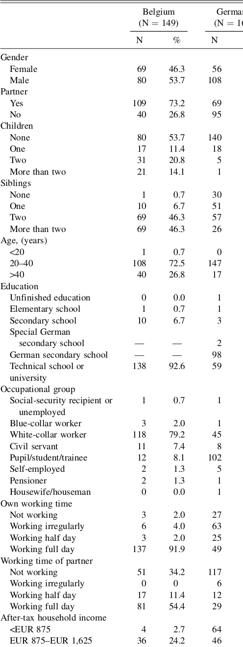
Our samples consist of 149 respondents in Belgium and 164 in Germany. The questionnaire appeared on the Internet and was advertised through Web newsletters in both countries. Each respondent was offered the right to participate in a lottery, with an expected payoff equal to EUR 5. The Belgian sample was col-lected in April 2002, the German sample was colcol-lected in Feb-ruary 2005. Table 1 presents a breakdown of the sample statistics for both countries. The gender distribution of the German sample is relatively male biased. In both countries, most respondents Koulovatianos, Schro¨der, and Schmidt: Nonmarket Household Time and the Cost of Children 43
were from 20 to 40 years of age and were highly educated. These biases are related to the distribution of Internet user attributes.
3. EQUIVALENT-INCOME PROFILES AND TIME/ MONEY TRADEOFFS
3.1 Descriptive Statistics
Table 2 presents the sample means of the stated equivalent incomes. An immediate observation is that respondents always compensate households for a reduction in NMTE. This is a plausible result, consistent with predictions by theories of the value of time in the literature.
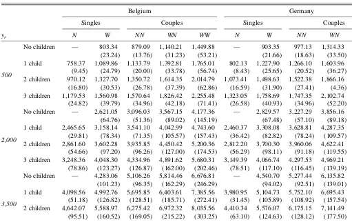
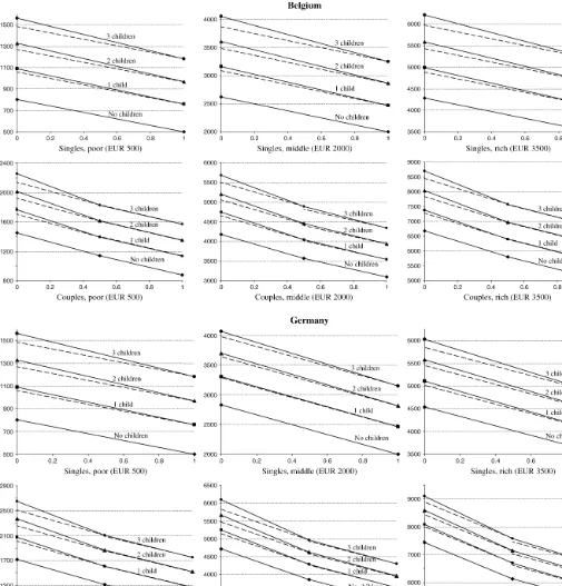
Figure 1 depicts the information given by Table 2. The hori-zontal axis of each graph represents a household’s available NMTE. The value 1 on the horizontal axis is for the case when all adults in the household are nonworking. The value 0 means that all adults in the household work full time. For the case of two-adult households in which one two-adult is working and the other is nonworking, the value 0.5 is assigned. The vertical axis is used for equivalent incomes. Each point plotted represents an average equivalent income, with one point for each mixture of household characteristics (given in Table 2). For example, consider the entry ‘‘WN,yr¼500, 2 children’’ for Belgium in Table 2. There we have the average equivalent income of EUR 1,614.35 for a couple with two children where one adult is working and the other is nonworking (reference income of EUR 500). This entry is plotted with amsymbol, which is in the middle of the line labeled ‘‘2 children’’ on the graph ‘‘Couples, poor (EUR 500)’’ in Figure 1. For any given family type presented in Figure 1, solid lines connect equivalent incomes that correspond to particular levels of NMTE. All solid lines in Figure 1 are downward sloping. This implies that, in both countries, for any given family type, a reduction in NMTE is always associated with a positive income compensation that captures the time/money tradeoff. Figure 1 also shows that as the number of children increases, equivalent incomes increase as well.
In each of the 12 graphs of Figure 1, the dashed lines are the ‘‘No children’’ lines, shifted upward in a parallel manner. Differences between slopes of dashed and solid lines reveal differences in the time/money tradeoff between families with children versus families without children. In both countries, the dashed lines that correspond to couples and a reduction in NMTE from 1 to 0.5 are hardly distinguishable from the solid lines. So, the time/money tradeoff is not affected by the pres-ence of children in the case of a nonrestrictive reduction in NMTE: a transition from NNto WN. On the contrary, when reductions in NMTE are restrictive (transition fromNtoWor fromWNtoWW), solid lines are steeper than dashed lines. This means that the presence of at least one child increases the time/ money tradeoff in response to a restrictive reduction in NMTE.
3.2 Testing the Effect of Children on Time/Money Tradeoffs
Table 3 presents statistical tests of the pattern revealed by the comparison of solid lines and dashed lines in Figure 1. The symbols
N!W,NN!WN, andWN!WWdenote a transition from a particular constellation of labor market participation of adults in a household to another constellation. The reduction in NMTE im-plied byNN!WNis nonrestrictive, whereasN!WandWN!
Table 1. Personal characteristics of respondents Belgium
(N¼149)
Germany (N¼164) N % N % Gender
Female 69 46.3 56 34.1 Male 80 53.7 108 65.9 Partner
Yes 109 73.2 69 42.1 No 40 26.8 95 57.9 Children
None 80 53.7 140 85.4 One 17 11.4 18 11.0 Two 31 20.8 5 3.0 More than two 21 14.1 1 0.6 Siblings
None 1 0.7 30 18.3 One 10 6.7 51 31.1 Two 69 46.3 57 34.8 More than two 69 46.3 26 15.8 Age, (years)
<20 1 0.7 0 0.0 20–40 108 72.5 147 89.6 >40 40 26.8 17 10.4 Education
Unfinished education 0 0.0 1 0.6 Elementary school 1 0.7 1 0.6 Secondary school 10 6.7 3 1.8 Special German
secondary school — — 2 1.2 German secondary school — — 98 59.8 Technical school or
university
138 92.6 59 36.0 Occupational group
Social-security recipient or unemployed
1 0.7 1 0.6 Blue-collar worker 3 2.0 1 0.6 White-collar worker 118 79.2 45 27.4 Civil servant 11 7.4 8 4.8 Pupil/student/trainee 12 8.1 102 62.4 Self-employed 2 1.3 5 3.0 Pensioner 2 1.3 1 0.6 Housewife/houseman 0 0.0 1 0.6 Own working time
Not working 3 2.0 27 16.5 Working irregularly 6 4.0 63 38.4 Working half day 3 2.0 25 15.2 Working full day 137 91.9 49 29.9 Working time of partner
Not working 51 34.2 117 71.3 Working irregularly 0 0 6 3.7 Working half day 17 11.4 12 7.3 Working full day 81 54.4 29 17.7 After-tax household income
<EUR 875 4 2.7 64 39.0 EUR 875–EUR 1,625 36 24.2 46 28.0 EUR 1,625–EUR 2,375 28 18.8 24 14.6 EUR 2,375–EUR 3,125 41 27.5 18 11.0
$EUR 3,125 40 26.8 12 7.4
44 Journal of Business & Economic Statistics, January 2009
WWimply restrictive reductions in NMTE. Table 3 presents com-pensations for specific reductions in NMTE by family type. Differ-ences in these compensations resulting from the presence of more children reflect differences in the slopes of solid lines in Figure 1.
To test for the effect of children on time/money tradeoffs, we investigated the statistical significance of differences in com-pensations for reductions in NMTE as the number of children increases. For each reference income, at the bottom and between each two consecutive columns of descriptive statistics in Table 3, appears a Wilcoxon signed-ranks test statistic and itsp value. It tests the equality of medians that correspond to these adjacent columns. The reason to use Wilcoxon signed-ranks tests instead of pairwiset tests is that normality is not guaranteed for the errors of the sample means, as seen by the descriptive statistics presented in Table 3. Because the com-pared observations come from the same sample of respondents, they are not independent. For this reason, differences in com-pensations for reductions in NMTE stated by each individual are tested against a zero-value null hypothesis.
The Wilcoxon tests support the pattern seen in Figure 1. In all cases of restrictive reductions in NMTE, children are associated with a stronger time/money tradeoff. In particular, in almost all of these cases, the presence of each additional child increases this tradeoff. On the contrary, if the reduction in NMTE is nonrestrictive, children typically do not affect time/ money tradeoffs; if they do, their impact on these tradeoffs is quantitatively smaller compared with restrictive reductions in NMTE (this small impact can also be seen in Figure 1).
Our results indicate that time for child-related activities is an essential component of child costs. This is corroborated by research based on time–use data. According to Gronau and Hamermesh (2006, p. 5, table 1), besides sleep, child-care is the second most time-intensive activity after leisure. Bradbury (2005) shows that parents reduce their leisure time considerably to raise their children. Fully working par-ents (W and WW) must either reduce their already limited leisure even more, or buy childcare and other housework services in the market. Traditional households (WN) may still accommodate the time component of child-related activities. For example, as noted by Apps and Rees (2001), the non-working partner can specialize in these activities. The role of time for child-related activities has a general implication for child costs that is consistent with Figure 1 and the tests appearing in Table 3: Child costs should be higher in time-constrained families when compared with households in which at least one adult is nonworking. In Section 4 we estimate child costs conditional upon the NMTE of adults, and test for this implication.
4. LABOR MARKET PARTICIPATION STATUS OF ADULTS AND CHILD COSTS
The regression analysis in this section has two purposes. First, it checks the robustness of the results presented in Section 3 by controlling for respondents’ personal characteristics. Sec-ond, the regressions provide estimates of child costs conditional
Table 2. Average stated equivalent incomes (values in Euros)
Belgium Germany
Singles Couples Singles Couples
yr N W NN WN WW N W NN WN WW
500
No children — 803.34 (23.24)
No children — 2,621.05 (64.76)
No children — 4,283.06 (101.23)
NOTE: Standard errors in parentheses.yrdenotes the level of reference income in Euros; eachNdenotes a nonworking adult, eachWdenotes a (full-time) working adult.
Koulovatianos, Schro¨der, and Schmidt: Nonmarket Household Time and the Cost of Children 45
upon the labor market participation status of adults after con-trolling for household-size economies.
The first regression model that follows Banks and Johnson (1994) and will serve as benchmark is
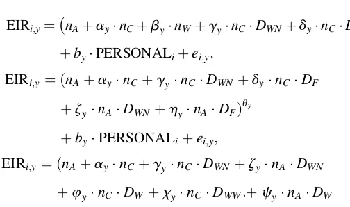
EIRi;y¼ nAþaynCþbynW uy
þbyPERSONALiþei;y: (1)
The variable EIRi,y is an equivalent-income ratio. It is the equivalent income stated by respondenti, divided by the ref-erence income,y, of a nonworking, single, childless adult. The
variablenAis the number of adults,nCis the number of chil-dren, andnWis the number of working adults in the household. So, nA, nW, and nC define the household type. Parameter uy controls for household-size economies at reference incomey. Dividing the stated equivalent income by the corresponding reference income (i.e., using EIRi,yas the dependent variable) will give estimates of parametersay,by, anduythat are com-parable across different reference incomes,y. Parameterbyis the compensation for a reduction in NMTE relative to the cost of a nonworking adult. Parameteray gives the cost of a
Figure 1. Equivalent incomes as functions of nonmarket time endowments. In each of the 12 graphs, the dashed lines are the ‘‘No children’’ lines shifted upward in a parallel manner to stress the change in the time/money tradeoff resulting from the presence of children. Reference incomes appear in parentheses.
46 Journal of Business & Economic Statistics, January 2009
Table 3. Stated compensation for different types of reduction in nonmarket time endowment ([NMTE] values in Euros)
Belgium
Singles Couples
N!W(restrictive reduction in NMTE) NN!WN(nonrestrictive reduction in NMTE) WN!WW(restrictive reduction in NMTE)
yr No children 1 child 2 children 3 children No children 1 child 2 children 3 children No children 1 child 2 children 3 children
500 Mean 303.34 331.49 357.58 381.45 261.11 259.02 263.63 255.78 309.67 372.20 400.44 429.07
Median 250.00 250.00 275.00 300.00 150.00 150.00 150.00 150.00 200.00 250.00 250.00 300.00
Standard error (23.24) (22.72) (24.56) (28.07) (24.57) (25.26) (26.27) (23.50) (28.30) (31.17) (34.94) (39.73)
Wilcoxon 3.53a 4.53a 2.78a 0.50 0.77 0.39 5.41a 3.18a 4.01a
pvalue [0.00] [0.00] [0.01] [0.62] [0.44] [0.70] [0.00] [0.00] [0.00]
2,000 Mean 621.05 692.49 740.68 799.94 471.11 501.89 514.56 556.66 610.21 700.61 749.95 788.68
Median 400.00 500.00 500.00 500.00 250.00 250.00 250.00 250.00 300.00 500.00 500.00 500.00
Standard error (64.76) (70.41) (75.30) (81.77) (61.94) (66.32) (69.99) (84.01) (68.70) (70.32) (73.10) (74.60)
Wilcoxon 4.31a 4.00a 5.13a 1.93c 0.73 2.69a 6.20a 4.31a 4.52a
pvalue [0.00] [0.00] [0.00] [0.05] [0.46] [0.01] [0.00] [0.00] [0.00]
3,500 Mean 783.06 894.19 946.90 1,021.98 708.19 707.77 696.90 722.42 862.36 981.95 1,063.24 1,130.31
Median 500.00 500.00 500.00 500.00 300.00 300.00 300.00 300.00 500.00 500.00 500.00 600.00
Standard error (101.23) (105.82) (110.61) (118.70) (107.56) (106.56) (105.83) (109.54) (107.45) (116.76) (126.65) (132.15)
Wilcoxon 6.40a 4.25a 3.90a 0.76 0.94 0.28 5.67a 5.16a 5.1a
pvalue [0.00] [0.00] [0.00] [0.45] [0.34] [0.78] [0.00] [0.00] [0.00]
Germany
500 Mean 403.35 425.76 425.21 435.64 337.20 337.87 343.78 355.47 401.52 466.62 505.03 542.83
Median 312.50 350.00 350.00 350.00 250.00 250.00 250.00 250.00 250.00 300.00 325.00 350.00
Standard error (21.66) (22.95) (25.48) (28.12) (24.85) (26.26) (28.15) (34.20) (29.06) (29.59) (31.95) (34.91)
Wilcoxon 2.26b 0.64 1.24 0.97 0.91 0.67 7.01a 5.14a 4.92a
pvalue [0.02] [0.52] [0.21] [0.33] [0.36] [0.50] [0.00] [0.00] [0.00]
2,000 Mean 829.57 847.71 888.11 917.35 628.87 658.54 662.35 671.68 862.44 962.20 1,038.35 1,122.87
Median 500.00 500.00 500.00 500.00 500.00 500.00 500.00 500.00 500.00 575.00 625.00 750.00
Standard error (67.48) (68.75) (73.09) (78.28) (59.94) (63.23) (64.58) (65.14) (86.14) (91.39) (97.50) (105.26)
Wilcoxon 4.22a 4.03a 3.36a 2.96a 1.23 1.83c 7.27a 5.68a 5.88a
pvalue [0.00] [0.00] [0.00] [0.00] [0.22] [0.07] [0.00] [0.00] [0.00]
3,500 Mean 1,040.70 1,123.78 1,165.73 1,212.50 858.38 943.32 966.34 988.60 1,296.49 1,382.16 1,451.34 1,518.29
Median 500.00 700.00 725.00 750.00 500.00 500.00 500.00 500.00 875.00 1,000.00 1,000.00 1,000.00
Standard error (94.02) (100.14) (105.44) (110.51) (85.63) (94.53) (97.95) (101.58) (131.09) (135.11) (139.05) (142.21)
Wilcoxon 5.24a 3.97a 4.93a 3.97a 2.28ab 2.70a 5.78a 5.44a 4.57a
pvalue [0.00] [0.00] [0.00] [0.00] [0.02] [0.01] [0.00] [0.00] [0.00]
NOTE: yrdenotes the reference income in Euros.
aSignificant at the 1% level.bSignificant at the 5% level.cSignificant at the 10% level.
Koulova
tianos,
Schro
¨der,
and
Schmidt:
Nonmarket
Household
Time
and
the
Cost
of
Children
47
child relative to a nonworking adult. PERSONALiis a set of conditioning variables that embrace the personal characteristics of respondentilisted in Table 1. Finally,ei,yis the error term. Columns labeled ‘‘Spec. 1’’ in Table 4 show the regression results for the benchmark specification (1). In both countries and for all reference incomes,byis greater thanay. This means that the compensation of an adult for working full time is greater than the cost of a child.
We extend the benchmark regression (1) to test the results of Section 3 using the three following regression models:
EIRi;y¼ nAþaynCþbynWþgynCDWNþdynCDF uy
þbyPERSONALiþei;y; ð2Þ
EIRi;y¼ ðnAþaynCþgynCDWNþdynCDF
þzynADWNþhynADFÞ uy
þbyPERSONALiþei;y; ð3Þ
EIRi;y¼ ðnAþaynCþgynCDWNþzynADWN
þuynCDWþxynCDWW:þcynADW
þvynADWWÞ
uyþb
yPERSONALiþei;y: ð4Þ
These models introduce the following four dummy variables: 1. DWNtakes the value 1 for a traditional household (WN,
either with or without children).
2. DFtakes the value 1 for eitherWorWWhouseholds (the symbol DF denotes the status of full labor market par-ticipation).
3. DWtakes the value 1 forW. 4. DWWtakes the value 1 forWW.
Specification (2) extends (1) by distinguishing the effect of a nonrestrictive versus a restrictive reduction in NMTE on child costs. The effect of a nonrestrictive reduction in NMTE is captured by including the interactionnCDWN, whereasnCDF captures the other effect. Specification (3) extends (2) by adding a distinction of the effect of a nonrestrictive versus a restrictive reduction in NMTE on the costs of adults—the inclusion ofnADWNandnADF(which necessitates dropping
nW). UsingDWandDWW, (4) further distinguishes the effects of restrictive reductions in NMTE on singles versus couples.
The estimates of (2) through (4) are presented in columns ‘‘Spec. 2’’ through ‘‘Spec. 4’’ of Table 4. The pattern seen in Figure 1 and tested in Table 3 is reconfirmed: Child costs are higher in time-constrained families compared with households in which at least one adult is nonworking. This can be seen by the general pattern that, in most cases, gy is statistically insignificant whereas dy, oruy andxy, are significant. In the two exceptions when gy is significantly positive, its value is smaller than the estimates ofuyandxy.
Two further results are of interest. The estimates of zyare always lower than these ofhy, orcyandvy. This comparison indicates that the traditional household is able to achieve gains from specialization not only with respect to child-related activities (as gy< xy implies), but also with respect to other home activities (see Apps and Rees 2001). Moreover, as in Koulovatianos et al. (2005), the estimates ofuyare seen to fall
with reference income, implying that the rich exhibit a higher ability to share within the household. This property has received both theoretical attention and empirical support (see Donaldson and Pendakur 2004, 2006).
All reported estimates in Table 4 are controlled for respon-dents’ personal characteristics. Although the inclusion of per-sonal characteristics adds some explanatory power to the regressions (it increasesR2), it does not alter the levels of the reported estimates. None of the personal characteristics appeared robust, so they are not reported in Table 4. (These results can be provided by the authors upon request.)
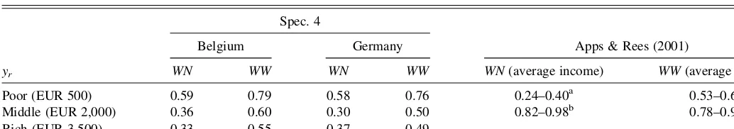
Table 5 presents a summary of ranges of child costs based on estimates of (4) compared with estimates by Apps and Rees (2001) for couples. In Apps and Rees (2001, p. 645), the sum of time costs and purchased goods for child-related activities is about 78% to 98% of the total consumption of an adult male. These numbers are higher than ours. This difference may be the result of (a) the particular assumptions concerning within-household sharing rules and within-household production functions that enable identification of the Apps-Rees demand system; and (b) the fact that, for our survey, respondents were instructed to consider children of age 7 to 11 years, who may require less childcare time than preschoolers (Bradbury 2005, pp. 20–21). Nevertheless, our questionnaire can be modified to focus on preschoolers in future research.
5. POLICY IMPLICATIONS FOR CHILD TAX ALLOWANCES
Estimating equivalent incomes of families with children contingent upon the labor market participation status of adults has important implications not only for antipoverty policies, but also for policies to reduce unemployment. For example, accord-ing to Table 2, a saccord-ingle nonworkaccord-ing parent of one child in Ger-many would need to receive EUR 802 monthly to be at the same level of well-being as that of a single, childless adult living on social assistance (who receives about EUR 500). These numbers imply equitable social assistance for these two family types.
If this single parent was, instead, working, then the equivalent disposable monthly income is about EUR 1,228, according to the estimates of Table 2. This number helps to understand the pos-sibility faced by low-income single parents of falling into an unemployment trap: EUR 1,228 corresponds to the 31st per-centile of the German disposable income distribution of single parents with one child in year 2003 (calculations based on the most recent German Income and Expenditure Survey ‘‘Einkommens-und Verbrauchsstichprobe’’). Thus, to provide work incentives to a single parent of one child, the tax/transfer system needs to ensure that the disposable income of this parent is higher than EUR 1,228, conditional upon the fact that this parent works.
In some countries, the link between parenthood and work incentives is taken into account. The income transfer systems for low-income families—the earned income tax credit (EITC) in the United States and the working families’ tax credit (WFTC) in the United Kingdom—condition tax credits on the labor market participation status of parents. For example, WFTC is higher if families work longer hours in the labor market (at least 30 hours per week), and WFTC is increasing in the number of dependent children (see Brewer 2001 for further 48 Journal of Business & Economic Statistics, January 2009
Table 4. Regressions for estimating child costs
Belgium
yr¼500 yr¼2,000 yr¼3,500
yr Spec. 1 Spec. 2 Spec. 3 Spec. 4 Spec. 1 Spec. 2 Spec. 3 Spec. 4 Spec. 1 Spec. 2 Spec. 3 Spec. 4
ay nC 0.67a(0.03) 0.59a(0.03) 0.57a(0.03) 0.59a(0.03) 0.44a(0.03) 0.37a(0.03) 0.35a(0.03) 0.36a(0.03) 0.39a(0.03) 0.34a(0.03) 0.32a(0.03) 0.33a(0.03)
by nW 0.91a(0.05) 0.75a(0.06) — — 0.64a(0.05) 0.51a(0.06) — — 0.57a(0.05) 0.48a(0.06) — —
gy nCDWN — 0.03 (0.04) 0.03 (0.05) 0.06 (0.06) — 0.01 (0.05) 0.08 (0.06) 0.13c(0.07) — 0.01 (0.05) 0.05 (0.07) 0.10 (0.08)
dy nCDF — 0.11 a
(0.04) 0.11a(0.04) — — 0.11a(0.04) 0.11a(0.04) — — 0.07 (0.05) 0.07 (0.05) —
zy nADWN — — 0.30a(0.04) 0.32a(0.05) — — 0.17a(0.03) 0.18a(0.05) — — 0.16a(0.05) 0.18a(0.06)
hy nADF — — 0.74a(0.06) — — — 0.51a(0.05) — — — 0.48a(0.06) —
uy nCDW — — — 0.10b(0.05) — — — 0.10b(0.05) — — — 0.07 (0.06)
xy nCDWW — — — 0.20b(0.09) — — — 0.24b(0.11) — — — 0.22c(0.12)
cy nADW — — — 0.75a(0.06) — — — 0.48a(0.07) — — — 0.42a(0.08)
vy nADWW — — — 0.77a(0.06) — — — 0.51a(0.08) — — — 0.49a(0.09)
uy — 0.85 a
(0.02) 0.88a(0.02) 0.88a(0.02) 0.85a(0.02) 0.68a(0.02) 0.69a(0.02) 0.70a(0.02) 0.66a(0.03) 0.63a(0.02) 0.64a(0.02) 0.64a(0.02) 0.59a(0.03)
R2 0.44 0.44 0.44 0.44 0.32 0.32 0.32 0.33 0.31 0.31 0.31 0.31
Germany
ay nC 0.64a(0.03) 0.57a(0.03) 0.55a(0.03) 0.58a(0.03) 0.36a(0.02) 0.32a(0.02) 0.30a(0.02) 0.30a(0.02) 0.26a(0.02) 0.23a(0.02) 0.21a(0.02) 0.19a(0.02)
by nW 0.95a(0.04) 0.82a(0.05) — — 0.77a(0.05) 0.66a(0.06) — — 0.68a(0.04) 0.59a(0.05) — —
gy nCDWN — 0.03 (0.04) 0.02 (0.05) 0.05 (0.05) — 0.04 (0.04) 0.03 (0.05) 0.07 (0.06) — 0.03 (0.04) 0.07 (0.05) 0.18a(0.07)
dy nCDF — 0.08a(0.03) 0.08b(0.03) — — 0.07c(0.04) 0.07c(0.04) — — 0.06c(0.03) 0.06c(0.03) —
zy nADWN — — 0.34a(0.04) 0.37a(0.04) — — 0.24a(0.04) 0.27a(0.05) — — 0.18a(0.04) 0.21a(0.05)
hy nADF — — 0.81a(0.05) — — — 0.66a(0.05) — — — 0.58a(0.05) —
uy nCDW — — — 0.09
b
(0.04) — — — 0.07 (0.05) — — — 0.12a(0.04)
xy nCDWW — — — 0.18b(0.07) — — — 0.20b(0.09) — — — 0.30a(0.11)
cy nADW — — — 0.80a(0.06) — — — 0.62a(0.07) — — — 0.40a(0.07)
vy nADWW — — — 0.86a(0.07) — — — 0.70a(0.08) — — — 0.71a(0.10)
uy — 0.93a(0.02) 0.96a(0.02) 0.96a(0.02) 0.92a(0.02) 0.72a(0.02) 0.74a(0.02) 0.75a(0.02) 0.70a(0.02) 0.66a(0.01) 0.68a(0.02) 0.68a(0.02) 0.58a(0.02)
R2 — 0.53 0.53 0.53 0.53 0.38 0.38 0.38 0.38 0.37 0.37 0.37 0.37
NOTE: Regressions for each reference income (yrdenotes the reference income level in Euros). Endogenous variable: equivalent-income ratio (i.e., equivalent income stated by respondents divided by the reference income of a nonworking, single,
childless adult). Number of observations: 2,831 in Belgium; 3,116 in Germany. White’s heteroscedasticity correction for covariance matrix; standard errors in parentheses. aSignificant at the 1% level.bSignificant at the 5% level.cSignificant at the 10% level.
Koulova
tianos,
Schro
¨der,
and
Schmidt:
Nonmarket
Household
Time
and
the
Cost
of
Children
49
details). In some U.S. states, EITC also increases with the number of children (see Neumark and Wascher 2007, p. 6).
The results presented here support the practice of the WFTC tax code to distinguish the hours worked by parents, as well as that of the EITC to increase benefits according to the number of children. These distinctions point in the right direction for increasing work incentives for parents. However, the empirical literature concerning the impact of EITC on unemployment is controversial. For example, the empirical literature typically finds evidence of positive effects of EITC benefits on the employment of parents (see Cancian and Levinson 2006, pp. 796–797 for a literature review), whereas Cancian and Levinson (2006) who focus on Wisconsin, where extra EITC supplements for families with children are provided, have found no such effect. It is therefore of critical importance to estimate the threshold income level that must be exceeded to provide sufficient work incentives for parents (such as our estimate of EUR 1,228 for single parents with one child in Germany). We believe we have shown how survey-based data can help to identify these thresholds.
6. CONCLUDING REMARKS
Childrearing requires parental time. Time–use data indicate that parents devote a substantial part of their leisure time to raise children. Consequently, working parents must either reduce their already limited leisure time even more or buy childcare and other housework services in the market. This means that parents may face additional opportunity costs upon deciding to start working full time. Children in the household can have an effect on the reservation wages of the adults.
We have designed a survey instrument to collect everyday people’s insights about the magnitude of income compensation required to maintain a constant level of family well-being when adults are working versus when they are nonworking. According to our survey respondents in Belgium and Germany, labor market participation compensation is higher when children are in the household, except for the case when only one of two nonworking parents decides to go to work. Consistently, our estimates of child costs are higher in time-constrained families compared with households where at least one adult is non-working.
Our study supports the view that policies channeling extra income tax allowances to working parents are likely to reduce the possibility that parents find themselves trapped in unem-ployment and poverty. Examples of such policies are the EITC in the United States and the WFTC in the United Kingdom.
ACKNOWLEDGMENTS
The authors are indebted to Irwin Collier and two anonymous referees for offering very detailed guidelines on how to craft this paper. They also thank Timm Bo¨nke, Martin Browning, Kath-arina Wrohlich, conference participants of the seventh meeting of the European Research Training Network (RTN) project on ‘‘The Economics of Ageing in Europe’’ in Venice, the workshop ‘‘Labour Markets and Demographic Change’’ in Rostock, and participants of the interdisciplinary seminar series at the Uni-versity of Vienna for useful comments and suggestions. Finan-cial support from the Training and Mobility of Researchers (TMR) network ‘‘Living Standards, Inequality and Taxation,’’ contract no. ERBFMRXCT980248, is gratefully acknowledged. C. K. thanks the Leventis foundation and the RTN project on ‘‘The Economics of Ageing in Europe’’ for financial support. U. S. acknowledges financial support from the Deutsche For-schungsgemeinschaft, contract no. Schm1396/1-1.
[Received August 2005. Revised March 2007.]
REFERENCES
Aiyagari, S., Greenwood, J., and Gu¨ner, N. (2000), ‘‘On the State of the Union,’’The Journal of Political Economy,108, 213–244.
Apps, P., and Rees, R. (2001), ‘‘Household Production,’’Full Consumption and the Costs of Children, Labour Economics,8, 621–648.
Banks, J., and Johnson, P. (1994), ‘‘Equivalence Scale Relativities Revisited,’’ The Economic Journal,104, 883–890.
Bradbury, B. 2005, ‘‘Time and the Cost of Children,’’ National Poverty Center Working Paper Series no. 05-4. Ann Arbor: University of Michigan. Brewer, M. (2001), ‘‘Comparing In-Work Benefits and the Reward to Work for
Families with Children in the US and the UK,’’Fiscal Studies,22, 41–77. Browning, M. (1992), ‘‘Children and Household Economic Behavior,’’Journal
of Economic Literature,30, 1434–1475.
Cancian, M., and Levinson, A. (2006), ‘‘Labor Supply Effects of the Earned Income Tax Credit: Evidence from Wisconsin’s Supplemental Benefit for Families with Three Children,’’National Tax Journal,59, 781–800. Donaldson, D., and Pendakur, K. (2004), ‘‘Equivalent-Expenditure Functions
and Expenditure-Dependent Equivalence Scales,’’Journal of Public Eco-nomics,88, 175–208.
——— (2006), ‘‘The Identification of Fixed Costs from Consumer Behavior,’’ Journal of Business & Economic Statistics,24, 255–265.
Greenwood, J., Seshadri, A., and Yorukoglu, M. (2005), ‘‘Engines of Liberation,’’The Review of Economic Studies,72, 109–133.
Gronau, R. (2006), ‘‘Home Production and the Macroeconomy: Some Lessons from Pollak and Wachter and from Transition Russia,’’ NBER Working Paper Series no. 8509. Cambridge, MA.
Gronau, R., and Hamermesh, D. (2006), ‘‘Time vs. Goods: The Value of Measuring Household Production Technologies,’’Review of Income and Wealth,52, 1–16. Koulovatianos, C., Schro¨der, C., and Schmidt, U. (2005), ‘‘On the Income Dependence of Equivalence Scales,’’Journal of Public Economics,89, 967–996. Neumark, D., and Wascher, W. 2007, ‘‘Minimum Wages, the Earned Income Tax Credit, and Employment: Evidence from the Post-Welfare Reform Era,’’ NBER Working Paper Series no. 12915. Cambridge, MA.
Table 5. Child costs relative to an adult inWNversusWWhouseholds
yr
Spec. 4
Apps & Rees (2001) Belgium Germany
WN WW WN WW WN(average income) WW(average income) Poor (EUR 500) 0.59 0.79 0.58 0.76 0.24–0.40a 0.53–0.69a Middle (EUR 2,000) 0.36 0.60 0.30 0.50 0.82–0.98b 0.78–0.91b Rich (EUR 3,500) 0.33 0.55 0.37 0.49
NOTE: yrdenotes the reference-income level in Euros.
aA model specification without considering household production and parental childcare. bA model specification considering household production and parental childcare.
50 Journal of Business & Economic Statistics, January 2009
Wooldridge, J. M. (2002),Econometric Analysis of Cross Section and Panel Data, Cambridge, MA: The MIT Press.
APPENDIX: SURVEY INSTRUMENT DOCUMENTATION
A.1 Purpose of the Survey
In general, different household types may need different income amounts to attain a given living standard. These income amounts may depend on the number of adults and children living in the household. Furthermore, household needs may depend on the labor-market-participation status of the adults (nonworking or working full time) since this might affect, for example, the time adults can spend for cooking or educating their children. Therefore, the following question arises:
Given the income of a specific household type (reference household), what is the income that can make another house-hold type (that differs with respect to the number of children and/or adults and/or number of working adults) attain an identical living standard as the reference household?
Since there does not exist an objectively correct answer, we would like to know your subjective assessment of this question.
A.2 Personal Characteristics
We would like to ask you to state some of your own personal characteristics. Please mark the boxes that apply to you. Your answers will be treated confidentially and only for the stated research purpose.
A.3 Income Assessment
In the tables below you shall evaluate three different sit-uations. These situations differ by the prespecified after-tax monthly income (including all social transfers) of a nonworking-single-childless-adult household. Now consider, for each sit-uation separately, that the size and composition of the house-holds change as indicated in the table.
Below, we give you an example of such a table. Please take some time to familiarize yourself with the structure of the table. Within a given table, all household types should attain the same living standard. Please, fill in the cells putting the after-tax/transfer family incomethat you believe brings the house-holds that differ with respect to the numbers of children, adults, and working adults, to the same living standard as the one of the nonworking single childless adult.
Please, complete the following three tables. For your assessment assume that adults are between 35 and 55 and children between 7 and 11 years old.
(Note to researcher: In the actual survey three tables having the same structure as below were provided, each for a different reference income in increasing order.)
1) Please state your gender: umale
ufemale 2) Are you living together with a partner? uyes
uno 2a) In case your answer to question 2) is ‘‘yes:’’
Is your partner working unot at all
upart time
ufull time
uirregularly? 3) How many children live in your
household? u0 u1
u2
u3 or more 4) What is yourafter-tax family income
per month? below 1.75P* u1.75P – 3.25P
u3.25P – 4.75P
u4.75P – 6.25P u6.25P and above
(*Note to researcher: P is the ‘‘poverty line’’ in a country (see Section 2 for details).)
5) Are you usocial security recipient
uunemployed
ublue-collar worker
uwhite-collar worker
ucivil servant
upupil, student, or
utrainee
uself-employed
upensioner
uhouseman/wife? 6) Are you working unot at all
upart-time
ufull-time uirregularly? 7) Please state your education level: uno degree
uelementary school
usecondary school
utechnical school or university 8) Please state the number of siblings you
lived together with during your childhood: u0
u1
u2
u3 or more 9) Please mark the correct age category you
belong to: ubelow 20 years
u20–40 years
u40 years and older
1 adult, nonworking
1 adult, working full time
2 adults, both nonworking
2 adults, 1 nonworking, 1 working full time
2 adults, both working full time 0 children Reference income
1 child 2 children 3 children
Koulovatianos, Schro¨der, and Schmidt: Nonmarket Household Time and the Cost of Children 51
![Table 3. Stated compensation for different types of reduction in nonmarket time endowment ([NMTE] values in Euros)](https://thumb-ap.123doks.com/thumbv2/123dok/1122740.761248/7.678.45.753.84.518/table-stated-compensation-different-reduction-nonmarket-endowment-values.webp)