Full Terms & Conditions of access and use can be found at
http://www.tandfonline.com/action/journalInformation?journalCode=ubes20
Download by: [Universitas Maritim Raja Ali Haji] Date: 11 January 2016, At: 19:29
Journal of Business & Economic Statistics
ISSN: 0735-0015 (Print) 1537-2707 (Online) Journal homepage: http://www.tandfonline.com/loi/ubes20
Density-Tempered Marginalized Sequential Monte
Carlo Samplers
Jin-Chuan Duan & Andras Fulop
To cite this article: Jin-Chuan Duan & Andras Fulop (2015) Density-Tempered Marginalized Sequential Monte Carlo Samplers, Journal of Business & Economic Statistics, 33:2, 192-202, DOI: 10.1080/07350015.2014.940081
To link to this article: http://dx.doi.org/10.1080/07350015.2014.940081
Accepted author version posted online: 25 Sep 2014.
Submit your article to this journal
Article views: 153
View related articles
Density-Tempered Marginalized Sequential
Monte Carlo Samplers
Jin-Chuan D
UANBusiness School, Risk Management Institute, National University of Singapore, Singapore ([email protected])
Andras F
ULOPESSEC Business School, Avenue Bernard Hirsch B.P. 50105, 95021 Cergy-Pontoise Cedex, France ([email protected])
We propose a density-tempered marginalized sequential Monte Carlo (SMC) sampler, a new class of samplers for full Bayesian inference of general state-space models. The dynamic states are approximately marginalized out using a particle filter, and the parameters are sampled via a sequential Monte Carlo sampler over a density-tempered bridge between the prior and the posterior. Our approach delivers exact draws from the joint posterior of the parameters and the latent states for any given number of state particles and is thus easily parallelizable in implementation. We also build into the proposed method a device that can automatically select a suitable number of state particles. Since the method incorporates sample information in a smooth fashion, it delivers good performance in the presence of outliers. We check the performance of the density-tempered SMC algorithm using simulated data based on a linear Gaussian state-space model with and without misspecification. We also apply it on real stock prices using a GARCH-type model with microstructure noise.
KEY WORDS: Bayesian methods; MCMC; Particle filter.
1. INTRODUCTION
In the last decade, particle filtering, based on sequential im-portance sampling, has become a state-of-the-art technique in handling general dynamic state-space models (see Doucet, De Freitas, and Gordon2001for a review). While such algorithms are well adapted for filtering dynamic latent states based on some fixed model parameter value, full Bayesian inference over parameters remains a hard problem. In a recent contribution, Andrieu, Doucet, and Holenstein (2010) proposed the particle MCMC (PMCMC) method as a generic solution which runs an MCMC chain over parameters, and used a particle filter to marginalize out latent states and to determine the acceptance probability in the Metropolis-Hastings (MH) step. They showed that for any finite number of particles, the equilibrium distribu-tion of the Markov chain is the joint posterior of the parameters and the latent states. Compared with traditional MCMC schemes that augment the parameter space with the latent states, the PM-CMC method is easy-to-use and is applicable to a wide range of problems.1
However, PMCMC can be computationally costly as it needs to run the particle filtering algorithm for tens of thousands of pa-rameter sets. A recent stream of papers proposed ways to enlarge the applicability of PMCMC by using adaptive MH proposals and relying on algorithms that are parallelizable in terms of model parameters. The former makes the algorithm more ef-ficient, whereas the latter takes advantage of modern general purpose graphical processing units (GPUs) and massively par-allel computing architectures. Pitt et al. (2010) stayed within the
1See Fernandez-Villaverde and Rubio (2007) for an intuitive application of
particle filter within MCMC, and Flury and Shephard (2008) for a demonstration of the PMCMC approach for an array of financial and economic models.
PMCMC framework and advocated the use of adaptive MCMC kernels. An alternative approach is to define a sequential Monte Carlo (SMC) sampling scheme over the parameters where the latent states are approximately marginalized out using a particle filter. Chopin, Jacob, and Papaspiliopoulos (2013) and Fulop and Li (2013) were primarily concerned with sequential inference, and defined the sequence of targets over gradually expanding data samples, which allows them to conduct joint sequential inference over the states and parameters.
This article makes two contributions. First, we propose an al-ternative sequence of targets for the marginalized SMC routine. We set up a density-tempered bridge between the prior and the posterior that allows a smooth transition between the two dis-tributions. We show that with a proper choice of the tempering scheme, the algorithm is easy to implement and delivers exact draws from the joint posterior of the dynamic states and the model parameters. There are two advantages of our proposed density-tempered marginalized SMC sampler as compared to the sequentially expanding data approach, which are particu-larly important in analyzing real data using models that are likely misspecified. First, it provides a direct link between the prior and posterior, reflected in fewer resample-move steps in running the algorithm. Second, through a judicious choice of the tempering scheme as in Del Moral, Doucet, and Jasra (2012), one can have a better control of particle diversity, reflected in lower Monte Carlo errors. This article’s second contribution
© 2015American Statistical Association
Journal of Business & Economic Statistics
April 2015, Vol. 33, No. 2 DOI:10.1080/07350015.2014.940081
Color versions of one or more of the figures in the article can be
found online atwww.tandfonline.com/r/jbes.
192
rests in proposing a new method for tuning the number of par-ticles for the latent state through using a reinitialized density tempering that is more stable than the exchange step advocated by Chopin, Jacob, and Papaspiliopoulos (2013).
Our contributions are illustrated by two applications. First, we examine the performance using a simple linear Gaussian state-space model where the exact likelihood is available from the Kalman filter. We investigate the performance of different al-gorithms when data are simulated based on a correctly specified model as well as when outliers of different magnitude are added to the data sample. Our first finding is that while the expanding-data and density-tempered SMC procedures perform similarly for noncontaminated data, the density-tempered approach is much more robust to data contaminations. These results hold true regardless of whether the exact likelihood (from the Kalman filter) or the estimated likelihood (from the particle filter) is used. Our second finding suggests that our new method for tuning the number of state particles leads to substantially lower Monte Carlo errors than the exchange step method of Chopin, Jacob, and Papaspiliopoulos (2013). The key to this improvement is a better control of particle diversity achieved by tempering.
Our second application is a study using a nonlinear asym-metric GARCH model with microstructure noises. The model is estimated on the daily stock price data of 100 randomly se-lected firms in the CRSP database during the 2002–2008 period. Our results suggest that the density-tempered approach outper-forms the expanding-data approach, and our new state particle tuning method also yields more reliable results.
Our article joins a growing literature on using SMC tech-niques in the Bayesian estimation of financial and economic models that often work with the joint density of the latent states and model parameters. For example, Jasra et al. (2011) estimated a stochastic volatility model using adaptive SMC samplers. In an online setting, Carvalho et al. (2010) provided methods to jointly estimate the model parameters and states for models that admit sufficient statistics for the posterior. Johannes, Korteweg, and Polson (2014) presented an application to predictability and portfolio choice. Herbst and Schorfheide (2014) developed an SMC procedure over parameters for macroeconomic mod-els where the likelihood function at fixed parameters is exactly known. Durham and Geweke (2011) investigated a GPU imple-mentation of expanding-data SMC samplers on a range of com-monly used models in economics. With our density-tempered SMC sampler, estimation and inference for a large class of com-plex state-space models can be reliably conducted.
2. ESTIMATION METHOD
We are concerned with the estimation of state-space models, where some latent variablesxtcompletely determine the future evolution of the system. Denote the model parameters byθ. The dynamics of the latent states is determined by a Markov process with the initial densityµθ(·) (i.e., forx1) and the transition
den-sityfθ(xt+1|xt). The observations{yt, t=1, . . . , T}are linked to the state of the system through the measurement equation
gθ(yt|xt). In what follows, for a given vector (z1, . . . , zt), we use the notationz1:t.
Our objective is to perform Bayesian inference over the latent states and model parameters conditional on the observations
y1:T. Ifp(θ) is the prior distribution overθ, the joint posterior is
In general, simulation-based methods are needed to sample from
p(θ, x1:T |y1:T).
2.1 An Overview of Pseudomarginal Approaches to Inference Using Particle Filter
Over the last 15 years, a considerable literature has been de-veloped on the use of sequential Monte Carlo methods (par-ticle filters) that provide sequential approximations to den-sities pθ(x1:t |y1:t) and likelihoods pθ(y1:t) for t =1, . . . , T at some fixed θ. Particle filters are ways to propagate a set of particles (representing the filtered distribution) over t by importance sampling and resampling steps.2 In particular, these methods sequentially produce sets of weighted particles
{(x1:(kt), wt(k)), k=1, . . . , M} whose empirical distribution
ap-Furthermore, the likelihood estimate is a byproduct:
ˆ Crucially for our purpose, these likelihood estimates have surprisingly good properties: (i) they are unbiased, that is,
E[ ˆpθ(y1:T)]=pθ(y1:T), where the expectation is taken with respect to all random quantities used in the particle filter (see Proposition 7.4.1 of Del Moral2004); and (ii) the variance of the estimates only increases linearly with sample size T (see Cerou, Del Moral, and Guyader2011).
The good behavior of the likelihood estimates suggests that it may be useful to take a hierarchical approach to the full inference problem by targeting the posterior density of the model param-etersp(θ |y1:T) and separately using a particle filter to estimate the necessary likelihoods p(y1:T |θ). Samples for the latent states at different time points will be obtained as a byproduct of the algorithm. This is exactly the pseudomarginal approach of Andrieu and Roberts (2008) that has been specialized to parti-cle filters by Andrieu, Doucet, and Holenstein (2010). The main point is that even though one cannot directly tacklep(θ|y1:T) due to the lack of a closed-form likelihood, the unbiasedness result opens a way of defining auxiliary variables whose joint
2For a general introduction to particle filters, readers are referred to Doucet and
Gordon (2001) whereas for the theoretical results, please see Del Moral (2004).
distribution withθadmits the target as marginal. Useut to de-note all random variables produced by a particle filter in step t. The corresponding joint density of these ensembles givenθ
for the whole sample isψ(u1:T |θ, y1:T). Now, extend the state-space to includeu1:T and define the auxiliary posterior as
˜
p(θ, u1:T |y1:T)∝pˆθ(y1:T)ψ(u1:T |θ, y1:T)p(θ). (5) Unbiasedness of the likelihood estimate means that the original target is a marginal distribution of the extended target as follows:
p(θ|y1:T)=
u1:T ˜
p(θ, u1:T |y1:T)du1:T. (6)
Furthermore, the original posterior shares the same normalizing constant as the extended posterior, which is exactly the marginal likelihood of the model:
There is a quickly growing family of methods that purport to draw from the extended target in (5). Particle MCMC methods, initiated by Andrieu, Doucet, and Holenstein (2010), propose to run a long Markov chain whose equilibrium distribution is
˜
p(θ, u1:T |y1:T).3A more recent set of algorithms, described in Chopin, Jacob, and Papaspiliopoulos (2013) and Fulop and Li (2013), propose to set up a sequence of densities on expanding data samples and to simulate a set of particles through this sequence using the iterated batch importance sampling (IBIS) routine of Chopin (2002). In particular, they work with the following sequence of expanding targets: fort=1, . . . , T,
The main rationale for this choice of targets is that each
πt(θ, u1:t) is an extended posterior over the data sample y1:t, hence the algorithm provides full sequential posterior inference which is the main objective of these methods. Note further that the algorithm also provides estimates ofZt, and hence sequen-tial marginal likelihoods can be computed.
In contrast to Chopin, Jacob, and Papaspiliopoulos (2013) and Fulop and Li (2013), this article is only concerned with batch inference and thus proposes an alternative sequence of densities based on a tempering bridge that can provide a more direct route to ˜p(θ, u1:T |y1:T) as compared to those expanding-data approaches.
2.2 Density-Tempered Marginalized SMC Sampler
The main idea of the SMC methodology is to begin with an easy-to-sample distribution and traverse through a sequence
3For recent extensions, see Pitt et al. (2010), Jasra, Beskos, and Thiery (2013),
Jasra, Lee, Zhang, and Yau (2013).
of densities to the ultimate target which is much harder to sample from. We construct a sequence of P densities be-tween π1(θ, u1:T)=p(θ)ψ(u1:T |θ, y1:T), and the extended posterior,πP(θ, u1:T)=p˜(θ, u1:T|y1:T), using a tempering se-quence {ξl;l=1, . . . , P}where ξl is increasing with ξ1=0
andξP =1. Note thatπ1(θ, u1:T) is easy to sample from and admits the prior over the fixed parameters as a marginal dis-tribution. The tempered sequence of targets is as follows: for
l=1, . . . , P,
The idea of tempering comes from Del Moral, Doucet, and Jasra (2006), but note that we only put the tempering term on the marginal likelihood estimate, ˆpθ(y1:T) as opposed to the entire quantity. This holds the key to the feasibility of our algorithm as will be shown later. Furthermore,πl(θ, u1:T), l < Pdoes not ad-mit the corresponding “ideal” bridging density [pθ(y1:T)]ξlp(θ) as a marginal, but this is of no consequence as the latter is of no independent interest. Next, as in Del Moral, Doucet, and Jasra (2006), we propagateNpoints through this sequence using se-quential Monte Carlo sampling. In the following, the superscript (i) always means for eachi=1, . . . , N.
2.2.1 Initialization. To begin atl=1, we need to obtain Nsamples fromπl(θ, u1:T)=ψ(u1:T |θ, y1:T)p(θ).
• Sampleθ(i)(1)∼p(θ) from the prior distribution over the
model parameters.
• To attachu(1:i)T(1), according toψ(u1:T |θ(i)(1), y1:T), run a particle filter for eachθ(i)(1) withMstate particles. To save for later use, store the estimate of the normalizing constant
ˆ
p(i)(1)=pˆθ(i)(1)(y1:T). Note that the random numbers used
in the particle filter are independent across samples and iterations.
• Attribute an equal weight,S(i)(1)=1/N, to each particle. The weighted sample at the (l−1)-stage of the iteration, that is, (S(i)(l−1), θ(i)(l−1), u(i)
1:T(l−1), i=1, . . . , N) rep-resents πl−1(θ, u1:T). With it, the algorithm goes through the following steps to advance to the next-stage representation of
πl(θ, u1:T).
2.2.2 Reweighting. Moving from πl−1(θ, u1:T) to
πl(θ, u1:T) can be implemented by reweighting the particles by the ratio of the two densities. This yields the following unnormalized incremental weights:
Importantly, the hard-to-evaluate density of the auxiliary ran-dom variables,ψ(u(1:i)T(l−1)|θ(i)(l−1), y
1:T), does not show up in the final expression.
Del Moral, Doucet, and Jasra (2012) noted that the tempering sequence can be adaptively chosen to ensure sufficient particle diversity. We follow their procedure and always set the next value of the tempering sequenceξlautomatically to ensure that the effective sample size (ESS)4 stays close to some constant B. This is achieved by a simple grid search, where the ESS is evaluated at the grid points of ξl, and the one with the ESS closest toBis chosen.
Finally, the weights are normalized to sum up to one and become
S(i)(l)= S(i)(l−1)˜s(i)(l)
N
j=1S(j)(l−1)˜s(j)(l)
.
2.2.3 Resampling. As one proceeds with the algorithm, the variability of the importance weights will tend to increase, leading to a sample impoverishment. To focus the computa-tional effort on areas of high probability, it is common in the sequential Monte Carlo literature to resample particles pro-portional to their weights. If ESS< B, one resamples the particles (θ(i)
(l−1), u(1:i)T(l−1), i=1, . . . , N) proportional to
S(i)(l−1) and after resampling, setS(i)(l−1)=N1.
2.2.4 Moving the Particles. With repeatedly reweighting and resampling, the support of the sample of the param-eters would gradually deteriorate, leading to a well-known particle depletion situation. Periodically boosting the sup-port is thus a must. For this, we resort to particle marginal Metropolis-Hastings moves as in Andrieu, Doucet, and Holen-stein (2010), and keep the target, γl(θ, u1:T), unchanged. A new particle (θ∗, u∗
1:T) is proposed using the proposal density
hl(θ∗|)ψ(u∗1:T |θ ∗, y
1:T). The importance weight needed for the MH move is
where ˆpθ∗(y1:T) is the marginalized likelihood estimate evalu-ated at (θ∗, u∗1:T). Note again that the density of the auxiliary variables,ψ(u∗1:T |θ∗, y1:T), falls out the final expression and hence does not need to be evaluated. The resulting MH move step looks as follows:
4ESS stands for effective sample size and is a commonly used measure of weight
variability. It is defined as ESS= N 1 i=1[S(i)(l−1)]2
where the weightsS(i)(l−1)
(i=1, . . . , N) sum up to 1. ESS varies between 1 andN, and a low value signals a sample where weights are concentrated on a few particles.
• Draw parameters fromθ∗ ∼h
l(·|θ(i)(l−1)) and run a par-ticle filter for eachθ∗withMstate particles. Compute the likelihood estimate ˆpθ∗(y1:T).
The marginal likelihood of the model, which is exactly ZP Z1, can
Our algorithm basically entails runningN particle filters in parallel, each with M particles. By the results of Del Moral, Doucet, and Jasra (2006), this algorithm provides consistent inference for the extended target ˜p(θ, u1:T|y1:T) asN goes to infinity.5 Given that the extended target admits our original targetp(θ|y1:T) as a marginal, the algorithm is an “exact ap-proximation” in the spirit of Andrieu and Roberts (2008); that is, it provides consistent inference on the marginal,p(θ|y1:T), for any given M state particles, as the number of param-eter particles, N, goes to infinity. When inference over the model parametersθis of interest, only the marginal likelihood
ˆ
pθ(i)(y1:T) and parameter θ(i) need to be stored. If one stores
the whole state particle path, the algorithm also provides full inference over the joint distribution p(θ, x1:T |y1:T), a direct consequence of the results in Andrieu, Doucet, and Holenstein (2010). In particular, they showed that the resulting extended density,N1pˆθ(y1:T)ψ(u1:T |θ, y1:T)p(θ), admits the joint poste-riorp(θ, x1:T |y1:T) as a marginal. A recent article by Jacob, Murray, and Rubenthaler (2014) shows a theoretical result that bounds the expected memory cost of the path storage and pro-poses an efficient algorithm to realize this.
Our algorithm can be trivially parallelized in the parameter dimension, a property that it shares with Chopin, Jacob, and Pa-paspiliopoulos (2013), Fulop and Li (2013), and particle MCMC with independent MH proposals as in Pitt et al. (2010). This is an important feature as it allows users to fully use the computational power of modern graphical processing units (GPUs) equipped with thousands of parallel cores. Lee et al. (2010) demonstrated how to speed up particle filters under a fixed parameter using GPUs when the number of particles becomes really large. They documented significant speedup when the number of particles, M goes to 10,000. In financial applications, however, one can often obtain a decent estimate of the likelihood with a couple of hundred state particles, which is not enough to keep all threads of the GPU occupied. Parallelizing the algorithm in the param-eter dimension is thus likely to better use the computing power. For this article, the SMC algorithm was coded in MATLAB whereas the particle filter was written in CUDA mex files to run on GPUs, where essentially each thread runs a particle filter corresponding to a fixed parameter value. Readers are referred to the Appendix of Fulop and Li (2013) for details of the CUDA implementation.
5For recent consistency results for the adaptive algorithm we use here and the
associated central limit theorems, see Jasra, Beskos, and Thiery (2013), Jasra, Lee, Zhang, and Yau (2013).
2.3 Tuning the Number of Particles
The number of state particles,M, is a key parameter deter-mining the efficiency of move steps in particle MCMC. Pitt et al. (2012) showed optimality of setting anM such that the Monte Carlo standard error of the likelihood estimator is around one. Now, we use this result to tuneMin our proposed density-tempered SMC method.
In the first stage, we run our density-tempered SMC algo-rithm with a moderate value of state particlesMI, and continue until the average acceptance rate drops below some prespeci-fied number,C.6Our main insight is that by var(ξln ˆp
θ(y1:T))=
ξ2var(ln ˆpθ(y1:T)), the Monte Carlo noise in our objective func-tion of the MH move is much reduced in the earlier move steps when the tempering parameter is small. Hence, the algorithm moves freely in the sample space even with a smallerMI. As the system is being heated up, this tempering parameter effect weakens. Increasing estimation errors in the likelihood target tend to decrease the acceptance rates. Denote the tempering pa-rameter at the stop time asξI and the mean of the parameter particles as ˆθI.
In the second stage, we continue the algorithm with a new but larger value ofM. Following Pitt et al. (2012), we aim to set the newMsuch that the standard error of the untempered likelihood estimator is around one. Operationally, we need to estimate the Monte Carlo error of the likelihood estimate at a reasonable value ofθ. Note that our initial parameter estimate, ˆθI, is a nat-ural candidate, because it can be interpreted as an approximate weighted maximum likelihood estimator which provides a con-sistent estimate ofθ0asTgoes to infinity.7Thus, we proceed to
estimate the variance of the likelihood by running independent particle filters usingMI particles at ˆθI.8Denote this variance estimator by σ2
MI( ˆpθ(y1:T)), and set the new number of state particles toMF ≈MI ×σM2I( ˆpθ(y1:T)). Next we need a valid way to transition fromMI toMF state particles in the SMC algorithm. Here there are at least two alternatives:
First, one could keep the existing θ population, run a new independent particle filter for eachθ(i)withMF state particles, and modify the weights to account for the change inM. This is exactly the exchange step proposed in Chopin, Jacob, and Pa-paspiliopoulos (2013). The argument implies that by attaching
incremental weights IW(i)=
rameter particle, it will be valid to continue the tempered SMC routine fromξIusing the newMF. Note that it is also important to adjust the estimate of marginal likelihood with the weighted average of these incremental weights,Ni=1IW(i)s˜(i)(l).
Unfor-tunately, we find that this exchange step in our applications can lead to large weight variability because the variance of IW(i)is hard to control, leading to increased Monte Carlo noise.
Instead, we propose to use a reinitialized tempering procedure to change M. First, fit some distribution Q(θ) to the existing
6Such a stopping criterion is taken from Chopin, Jacob, and Papaspiliopoulos
(2013).
7See, for example, Hu and Zidek (2002).
8In contrast, Pitt et al. (2012) suggested to run an initial short Markov Chain
with a largeM, compute the posterior mean ˆθ0, and estimate the variance of
likelihood by running independent particle filters at ˆθ0.
parameter particle population to encode the information that we have built up so far on the parameters. In the applications later, we use a flexible mixture of normals for this purpose. In general, the more flexibleQ(θ) is, the moreθ particles are needed to reliably estimate it. Next, new parameter particles are drawn fromQ(θ), and for each sampledθ, an independent particle filters withMF state particles is run, resulting in a joint density ofQ(θ)ψMF(u1:T |θ, y1:T). Evidently this proposal does not admit the ultimate posterior as a marginal, hence we link it to the extended target ˆpθ(y1:T)p(θ)ψMF(u1:T |θ, y1:T) through a sequence of tempered densities as follows:
γl(θ, u1:T)=Q(θ)1−ξl[ ˆpθ(y1:T)p(θ)]ξlψMF(u1:T |θ, y1:T)
γP(θ, u1:T) is exactly your eventual target—the full-sample pos-terior, andZP/Z1is the marginal likelihood if both the proposal
Q(θ) and the priorp(θ) integrates to 1 as densities should be. We can then run an adaptive density-tempered SMC algorithm on this sequence. Note thatQ(θ) is kept fixed throughout the tempering steps, that is, is not recalibrated.
3. APPLICATIONS
3.1 Linear Gaussian State-Space Model
To study the performance of the density-tempered SMC sam-pler, we start with a simple linear Gaussian state-space model where the likelihood is available in a closed form from the Kalman filter. The model is
study follows Flury and Shephard (2011) who used the same model to benchmark the performance of the PMCMC algo-rithm.
To ensure positive variances, we parameterize with the log of the variances. That is, takeθ=(µ,lnσ2
ε, φ,lnση2) and constrain
φ∈(−1,1) using a truncated prior for this parameter. We inves-tigate the performance of different SMC algorithms for (1) data in accordance with the model and (2) data being contaminated by outliers. In each scenario, we generateT =1000 observa-tions using parameter valuesθ∗=(0.5,ln(1),0.825,ln(0.75)). Then, a given observation is contaminated by noise equal to
Bt×ǫt,whereBt is a Bernoulli indicator with parameter 0.01 andǫtis normal with mean zero and standard deviationα. Note that α controls the degree of model misspecification and we consider the values in {0,5,10,15,20}; that is, we examine cases from no outliers to severe outliers. To focus on the role of simulation error by different algorithms, we simulate a single dataset in each scenario and compute statistics from 50 indepen-dent runs of each algorithm. We assume a Gaussian prior given
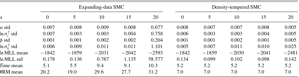
Table 1. Simulation results for the linear Gaussian state-space model with an exact likelihood
Expanding-data SMC Density-tempered SMC
α 0 5 10 15 20 0 5 10 15 20
µstd 0.007 0.008 0.009 0.008 0.677 0.008 0.007 0.007 0.008 0.005 lnσ2
ε std 0.007 0.003 0.003 0.004 0.758 0.006 0.003 0.003 0.004 0.005
φstd 0.001 0.001 0.002 0.002 0.204 0.001 0.001 0.002 0.001 0.005 lnσ2
ηstd 0.006 0.009 0.011 0.011 1.101 0.005 0.007 0.011 0.010 0.025
ln MLL mean −1842 −1859 −2031 −2042 −2593 −1842 −1859 −2030 −2041 −2481 ln MLL std 0.178 0.136 0.767 1.135 58.577 0.134 0.099 0.102 0.098 0.142 Time mean 5.1 5.5 9.4 9.1 10.3 5.2 5.2 5.2 5.2 5.2 #RM mean 20.2 19.0 29.6 27.7 31.2 7.0 7.0 7.0 7.0 7.0
NOTE: This table presents the results of a small Monte Carlo study of the linear Gaussian state-space model with different degrees of data contamination. For each scenario, a dataset of
T=1000 observations is generated using parameter valueθ∗=(0.5,ln(1),0.825,ln(0.75)), and random normal contaminations are added to the observations with probability 0.01, and
when happens, the noise has a standard deviationα. The statistics in the table are computed from 50 independent runs of the expanding-data and density-tempered SMC algorithms where the exact likelihood from the Kalman filter is used. The number of parameter particles isN=1024, and each time a move takes place, it takes 10 joint random walk MH moves. The first four rows report the standard deviation of posterior mean estimates of the parameters over the 50 independent runs. The fifth and sixth rows report the mean and standard deviation of the log of the marginal likelihood estimates over the 50 runs. The seventh and eighth rows report the average runtime in seconds and the average number of resample-move steps taken. The code was run on a Fermi M2050 GPU.
byθ∼N(θ0;I4),whereθ0=(0.25,ln(1.5),0.475,ln(0.475)),
and always use N =1024 parameter particles. The resample move step is triggered whenever the ESS drops belowB =N/2. A move step always takes 10 joint normal random walk moves where the variance of the innovations is set to dim(2.38θ2)Vˆlwith ˆVl being set to the estimated covariance matrix reflective of the current particle population.9
To zero in on the difference between the expanding-data and density-tempered SMC approaches, we compare the perfect marginalized algorithms that use the exact likelihood available from the Kalman filter. The first four rows ofTable 1report the standard deviation of the posterior mean parameter estimates over the 50 runs, whereas the fifth and sixth rows report the mean and standard deviation of the log of the normalizing con-stant (i.e., marginal likelihood) estimate, the seventh row the mean computing times (in seconds), and the eighth row the average number of resample move steps taken.10
The two columns corresponding to a correctly specified data generating process (i.e.,α=0) show that the standard devia-tions of the parameter estimates and the normalizing constants are similar for the two algorithms, and hence both provide re-liable inference in this case. Their computing times seem also comparable, which is a somewhat surprising result given that the initial resample-move steps for the expanding-data algorithm should take much less time because it processes a much smaller dataset. Our results show that this advantage is neutralized by a desirable feature of the density-tempered SMC sampler which needs significantly fewer resample-move steps to reach from the prior to the posterior (7 vs 20 as inTable 1). The tempering sequence provides a more direct link between the prior and the posterior as it is not forced through all the intermediate posteri-ors. Looking through the columns with increasingly prominent presence of outliers (growingα), the two algorithms starkly dif-fer. While the density-tempered approach provides stable results
9This is a standard approach in the adaptive MCMC literature; see, for example,
Andrieu and Thoms (2008) for a survey.
10The average of the posterior means are basically identical for the two
al-gorithms, apart from the most serious case of misspecification which the expanding-data algorithm is completely unreliable.
for all scenarios (though with some increased simulation noise), the Monte Carlo error of the expanding-data approach blows up as outliers become larger in magnitude. In essence, outliers lead to highly variable incremental weights in the reweighting step of the SMC algorithm, resulting in a poorly represented posterior. Moreover, the Monte Carlo error of the marginal likelihood esti-mates seem to deteriorate faster than the full-sample parameter estimates. This is understandable because the former reflects the approximation errors over the whole sequence of densities between the prior and posterior, whereas the latter only mea-sures the simulation error at the end, and by which stage the MCMC moves have corrected some of the intermediate errors. Finally, one observes that the number of resample-move steps and the computing time are quite stable for the density-tempered algorithm across the different scenarios, but the expanding-data approach takes substantially more move steps and need more computing time when outliers become more severe.
Next, we investigate the effect of using pseudomarginalized SMC algorithms by running the expanding-data and density-tempered SMC algorithms where approximate likelihoods are generated by a particle filter. For the linear Gaussian state-space model, the locally optimal importance proposalf(xt+1 |
xt, yt+1) is available analytically, and it is what we use in the
adapted particle filter. In all applications in this article we use stratified resampling within the particle filters. We fix the num-ber of state particle atM=512 for both algorithms. Other than this, the simulation setting is identical to the previous case. Over-all, the results inTable 2suggest that the two algorithms perform similarly when the model has no misspecification. However, the density-tempered SMC algorithm is much more stable for data with severe contamination. In general, we can observe larger Monte Carlo noises due to the use of an approximate likelihood, which is evident by comparingTable 2withTable 1.
Finally, we investigate how the two methods of setting the number of state particles performs on simulated data and report the results inTable 3. We simulate 50 datasets and each with
T =1000 observations. The data contamination is conducted with a probability 0.01 to add a normally distributed error with a standard deviation of 10. For each simulated dataset, 20 in-dependent runs of three variants of the density-tempered SMC
Table 2. Simulation results for the linear Gaussian state model with an approximate likelihood using a fixed number of state particles (M=512)
Expanding-data SMC Density-tempered SMC
α 0 5 10 15 20 0 5 10 15 20
µstd 0.011 0.006 0.014 0.025 1.408 0.009 0.007 0.025 0.030 0.024 lnσ2
ε std 0.008 0.004 0.007 0.031 0.821 0.007 0.004 0.010 0.014 0.016
φstd 0.001 0.001 0.002 0.005 0.173 0.001 0.001 0.004 0.005 0.018 lnσ2
ηstd 0.007 0.008 0.014 0.046 0.960 0.007 0.008 0.026 0.031 0.070
ln MLL mean −1842 −1859 −2031 −2044 −2623 −1842 −1859 −2030 −2041 −2481 ln MLL std 0.174 0.151 1.219 1.148 75.964 0.114 0.100 0.242 0.312 0.290 Time mean 239.6 262.8 491.8 473.6 518.2 300.0 299.8 315.9 343.4 317.9 #RM mean 20.3 19.3 30.0 27.9 30.6 7.0 7.0 7.2 7.9 7.6
NOTE: This table presents the results of a small Monte Carlo study of the linear Gaussian state-space model with different degrees of data contamination. For each scenario, a dataset ofT=1000 observations is generated using parameter valueθ∗=(0.5,ln(1),0.825,ln(0.75)), and random normal contaminations are added to the observations with probability 0.01,
and when happens, the noise has a standard deviationα. The statistics in the table are computed from 50 independent runs of the expanding-data and density-tempered SMC algorithms where the approximate likelihood from the adapted particle filter is used. The number of parameter particles isN=1024, and each time a move takes place, it takes 10 joint random walk MH moves. The first four rows report the standard deviation of posterior mean estimates of the parameters over the 50 independent runs. The fifth and sixth rows report the mean and standard deviation of the log of the marginal likelihood estimates over the 50 runs. The seventh and eighth rows report the average runtime in seconds and the average number of resample-move steps taken. The code was run on a Fermi M2050 CPU.
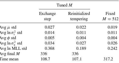
algorithms are carried out. Two of these variants adjustM as described in Section2.3. For each run, the algorithms are ini-tialized withMI =32 and the adjustment toMis triggered when the acceptance rate drops belowC=0.2.11The remaining algo-rithm is based on a fixed number of state particle atM=512. All other settings for the SMC algorithms are the same as in the previous case. The first column ofTable 3corresponds to using the exchange step of Chopin, Jacob, and Papaspiliopou-los (2013) to modifyM, whereas the second column is for the reinitialized tempering procedure proposed in this article. The functionQ(·) used in reinitialization is a six-component mix-ture of normals. The third column reports the results of the density-tempered SMCS with a fixedM=512. The first four rows report the average across the 50 datasets of the standard deviation of posterior mean estimates of the model parameters over the 20 independent runs of the algorithms. The fifth row reports the average standard deviation of the log marginal likeli-hood estimates, again the average is taken across the 50 datasets of the standard deviation over the 20 density-tempered SMC runs. The sixth row reports the average final number of state particlesM, whereas the seventh row gives the average runtime in seconds.
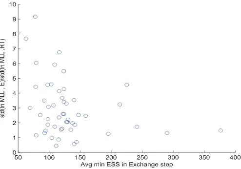
Comparing the second and third columns, it is clear that the algorithm with automatically adjustedMwith reinitialized tem-pering produces at least as reliable results as does the algorithm with a fixed M. Looking at the first and the second columns, one can conclude that the exchange step of Chopin, Jacob, and Papaspiliopoulos (2013) introduces considerable extra Monte-Carlo noise into the estimates, and it is particularly pronounced for the normalizing constant (i.e., marginal likelihood) esti-mates. The reason underlying this phenomenon is the occasional particle impoverishment due to the incremental weights intro-duced by the exchange step. For further illustration, we plot inFigure 1, a measure of particle impoverishment versus the extra Monte Carlo noise in the normalizing constant estimate due to the exchange step for each simulated dataset. To measure
11We take this value from Chopin, Jacob, and Papaspiliopoulos (2013).
particle impoverishment, we compute the minimum effective sample size (ESS) of the parameter particles during each SMC run with the exchange step. The horizontal axis in this plot is the average of the minimum ESS over the 20 independent runs of the SMC algorithm. The vertical axis is a measure of the extra Monte Carlo noise from the algorithm with the exchange step as compared to the algorithm with reinitialized tempering. Specifically, we compute the standard deviation of the log marginal likelihood estimates over the 20 runs for both
algo-Table 3. Simulation results for the linear Gaussian model by a density-tempered SMC algorithm with and without tuningM
TunedM
Exchange Reinitialized Fixed step tempering M=512
Avgµstd 0.027 0.022 0.019 Avg lnσ2
ε std 0.014 0.011 0.011
Avgφstd 0.005 0.004 0.004 Avg lnσ2
ηstd 0.034 0.027 0.026
Avg ln MLL std 0.368 0.189 0.242 Avg finalM 336 336
Time mean 108.7 107.1 317.2
NOTE: This table presents the results of a small Monte Carlo study of the linear Gaussian state-space model with and without tuning the number of state particleM. 50 datasets ofT=
1000 observations are generated using parameter valueθ∗=(0.5,ln(1),0.825,ln(0.75)),
and random normal contaminations are added to the observations with probability 0.01, and when happens, the noise has a standard deviation of 10. For each simulated dataset, we run 20 independent runs of three variants of the density-tempered SMC algorithm. The likelihood is approximated by an adapted particle filter throughout withMbeing adjusted according to the algorithm. The number of parameter particles isN=1024, and each time a move takes place, it takes 10 joint random walk MH moves. The first two columns report the results whereMis automatically adjusted using the approach described in Section
2.3. For each run, the algorithms are initialized withM=32, and an adjustment toMis triggered when the acceptance rate drops below 0.2. The first column corresponds to using the exchange step of Chopin et al. (2013) to modifyM, whereas the second column is for the reinitialized tempering procedure proposed in this article. The functionQ(·) used in reinitialization is a six-component mixture of normals. The third column reports the results of the density-tempered SMCS with a fixedM=512. The first four rows report the average across the 50 datasets of the standard deviation of posterior mean estimates of the model parameters over the 20 independent runs of the algorithms. The fifth row reports the average standard deviation of the log marginal likelihood estimates, again the average is taken across the 50 datasets of the standard deviation over the 20 density-tempered SMC runs. The sixth row reports the average final number of state particlesM, whereas the seventh row gives the average runtime in seconds. The code was run on a Fermi M2050 GPU.
Figure 1. Particle impoverishment versus Monte Carlo noise from the exchange step.
Note:Each point in this scatterplot represents the results for one of the 50 simulated datasets in the Monte Carlo study presented inTable 3. For each simulated dataset and each run of the SMC algorithm with the exchange step (described in Section2.3), we compute the mini-mum effective sample size of the parameter particles during the run. The horizontal axis is the average of the minimum ESS over the 20 independent runs of the SMC algorithm. The vertical axis is a measure of the extra Monte Carlo noise from the algorithm with the exchange step as compared to the algorithm with reinitialized tempering. Specifi-cally, we compute the standard deviation of the log marginal likelihood estimates over the 20 runs for both algorithms, and take the ratio of the standard deviations (exchange/reinitialized tempering).
rithms, and take the ratio of the standard deviations (exchange/ reinitialized tempering).
It is evident from this plot that for datasets where the SMC algorithm with the exchange step encounters phases with small ESSs, the normalizing factor estimate has a much higher vari-ance with the algorithm containing the exchange step as com-pared to the one with reinitialized tempering. Similar results hold for the parameter estimates. In unreported experiments, we have found that the SMC algorithm with the exchange step can be quite sensitive to the choice of the adjustment trigger,C, with lower values of the trigger leading to substantially higher Monte Carlo noise. For such cases, the tempering parameter at the adjustment tends to be larger, leading toward more variable incremental weights when moving to a newM. In contrast, reini-tialized tempering seemed quite robust to this choice and to the choice ofMI. The intuition is that the first stage of the algorithm only needs to provide a reasonable set of parameter particles and no information on the state particles is carried forward.
3.2 GARCH Model With Microstructure Noise
The purpose of this section is to demonstrate the applicabil-ity of the densapplicabil-ity-tempered SMC sampler on a typical nonlin-ear model in finance and to compare its performance with the expanding-data SMC sampler on real data. Here we consider the nonlinear asymmetric GARCH(1,1) (NGARCH) model of Engle and Ng (1993) with observation noise in a state-space
formulation. A similar model has been investigated in Pitt et al. (2010).
The logarithm of the observed stock price, denoted by Yt, often contains a transient componentZt, due to microstructure noises particularly for smaller and less liquid firms. Denoting the log “efficient” price by Et, the log observed price can be written as
Yt =Et+Zt. (9) The efficient price is assumed to have the following NGARCH dynamic and its innovations follow a generalized error distribu-tion:
Et−Et−1 =µ+σtεt (10)
σt2 =α0(1−α1)+α1σt2−1+β1σt2−1
×[(εt−1−γ)2−(1+γ2)] (11)
εt |Ft−1 ∼GED(v), (12)
where Ft stands for the information set available at time t and GED(v) is a generalized error distribution with mean 0, unit variance and tail-thickness parameter v >0.12 The den-sity of the GED(v) distribution isf(ε)= vexp[−
1 2|
ε λ|v] λ2(1+1/v)Ŵ(1/v), where
λ=[2(−2/v)Ŵ(1/v)/ Ŵ(3/v)]1/2. This family includes quite a
few well-known distributions; for example, v=2 yields the normal distribution andv=1 the double exponential distribu-tion. We use the results of Duan (1997) to impose the following sufficient conditions for positivity and stationarity of the vari-ance process:α0, α1, β1>0,α1−β1(1+γ2)>0 andα1<1.
We assume a constant signal-to-noise ratio, so the conditional volatility of the measurement noise,Zt, isδσt. The constantδis the ratio of the noise volatility over the signal volatility, that is, the inverse signal-to-noise ratio. To allow for the possibility of fat-tailed measurement noises, we assume that the standardized measurement noise has a generalized error distribution with tail thickness parameterv2. Hence, we have
Zt=δσtηtwhereηt ∼GED(v2) iid. (13)
We estimate the model on daily stock prices between 2002– 2008 of 100 randomly selected firms in the CRSP database. This in effect subjects different SMC algorithms to a wide range of data-generating processes and potential misspecifications. We exclude penny stocks (prices lower than 2 USD) and only use price data on actual transactions. Furthermore, we restrict the investigation to firms traded either on NYSE or NASDAQ, and having at least 1500 observations during the sample period.
The specifications of the independent priors for the model parameters are described inTable 4. As that table shows, for the two tail-thickness parameters –vandv2, we have assumed a
uniform prior over [1,2]; that is, transition innovations and mea-surement noises lie between the double exponential and normal distributions. For the other parameters, their distributions along with the 5th and 95th percentiles are given in Table 4. These percentile values are chosen with the intent to pick numbers that are relatively uninformative. For instance, the central 90%
12See Box and Tiao (1973) and Nelson (1991).
Table 4. Prior specification for the NGARCH model observed with noise
Density function 5th percentile 95th percentile
α0 Inverse Gamma Vi/5 Vi×5
α1 Beta 0.3 0.95
β1 Beta 0.01 0.3
γ Normal −3 3
µ Normal −1/252 1/252 v Uniform(1,2)
δ Gamma 0.01 1
v2 Uniform(1,2)
NOTE: This table summarizes the choice of the prior for the NGARCH model with noise.
Videnotes the observed variance of the returns,Yt−Yt−1for firmi.
prior interval for the daily mean returnµis [−1/252,1/252], corresponding to an annualized mean return in [−1,1], which arguably encompasses all economically relevant values of ex-pected stock returns.
The proposal sampler for the particle filter is the locally op-timal proposal under the Gaussian version of the model, but its standard deviation has been inflated by a factor of 1.2 to better cover the heavy-tailed distributions. For each firm, the conditional variance is initialized at the sample variance of the observed returns. For all SMC samplers over the model param-eters,N =4096 particles is deployed and the resample-move step is triggered atB =0.75N. We use a single joint move in the MCMC kernel and an independent proposal fitting a six-component normal mixture to the most recent population of parameter particles. Apart fromµandγ, we use the log trans-form to keep the proposal positive. Three SMC algorithms are investigated: expanding-data SMC with M=256 state parti-cles, density-tempered SMC withM=256 state particles, and density-tempered SMC withMtuned according to the reinitial-ized tempering described in Section2.3. In this latter case, the initial number of state particles is set toMI =64, and the ad-justment toM is triggered whenever the acceptance rate drops belowC=0.4. We choose a higher adjustment trigger because we expect the ideal acceptance probability to be higher with our mixture-of-normals MCMC proposal as compared to the sim-ple normal random walk proposal used in our earlier simulation study. A computer equipped with an Nvidia Tesla K20 GPU card is used to produce the results for this analysis.
The first and second columns ofTable 5contain results for the expanding-data and density-tempered SMC algorithm with a fixed M, whereas the third column reports the results using the density-tempered SMC algorithm with a tunedM. The first 16 rows are the averages across the 100 firms of the means and standard deviations of the posterior mean estimates for the parameters over 20 independent runs of an algorithm. It is evident from these results that the mean estimates from all three algorithms are close. However, the Monte Carlo noise of the expanding-data SMC algorithm is considerably larger than those of the density-tempered SMC variants. Furthermore, the tempered algorithm with a tunedM performs similarly to the one with a fixedM. The 17th row reports the average standard deviation of the log marginal likelihood estimates where again the average is taken across 100 firms of the standard deviations
Table 5. Estimation results for the NGARCH model observed with noise
(Expanding-data, (Tempered, (Tempered, fixedM) fixedM) tuningM)
Avgα0mean 0.0007 0.0008 0.0008 Avgα0std (0.0000) (0.0000) (0.0000) Avgα1mean 0.9504 0.9550 0.9559 Avgα1std (0.0017) (0.0010) (0.0008) Avgβ1mean 0.0906 0.0895 0.0901 Avgβ1std (0.0027) (0.0014) (0.0012) Avgγmean 0.5718 0.5680 0.5820 Avgγstd (0.0256) (0.0181) (0.0157) Avgµmean 0.0001 0.0001 0.0001 Avgµstd (0.0000) (0.0000) (0.0000) Avgvmean 1.1119 1.1125 1.1116 Avgvstd (0.0036) (0.0027) (0.0021) Avgδmean 0.1932 0.1863 0.1874 Avgδstd (0.0056) (0.0031) (0.0027) Avgv2mean 1.4630 1.4581 1.4625 Avgv2std (0.0238) (0.0162) (0.0142) Avg ln MLL std 0.6357 0.1679 0.0972 Time mean 731.7 148.5 150.4 # RM Mean 75.1 14.5 11.2+ 8.5
NOTE: This article presents the results for the NGARCH model with noise using daily stock prices between 2002–2008 of 100 randomly selected firms in the CRSP database. The first and second columns contain results for the expanding-data and density-tempered SMC algorithm with a fixedM=256, whereas the third column reports the results using the density-tempered SMC algorithm with a tunedM(initialized withM=64 and the adjustment toMis triggered when the acceptance rate drops below 0.4). All three algorithms useN=4096 parameter particles and an independent mixture of normals proposal with six components fitted on the parameter particles. The first 16 rows are the averages across the 100 firms of the means and standard deviations of the posterior mean estimates for the parameters over 20 independent runs of an algorithm. The 17th row reports the average standard deviation of the log marginal likelihood estimates where again the average is taken across 100 firms of the standard deviations over the 20 SMC runs for each algorithm. The 18th row reports the average runtime in seconds. The 19th row reports the average number of resample-move (RM) steps, where for the third column, we report both the average number of RM steps in the initial phase (before + sign) and final stage after tuningM(after + sign). The code was run on a Kepler K20 GPU.
over the 20 SMC runs for each algorithm. Similar to the re-sults obtained with the simulated examples, the advantage of the density-tempered SMC algorithm for estimating marginal likelihood is larger than for parameter estimates.
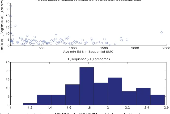
A crucial driver behind a larger Monte Carlo noise for the expanding-data SMC algorithm is that a few “too informative” observations can cause a collapse in particle diversity. The up-per panel ofFigure 2is used to illustrate this phenomenon by relating a measure of particle degeneracy for the expanding-data SMC algorithm to the Monte Carlo noise of the expanding-data SMC algorithm relative to the density-tempered SMC method. Each point on the scatterplot represents results of a single firm as inTable 5. For each dataset and each run of the expanding-data SMC algorithm, we compute the minimum effective sample size of the parameter particles during the run. The horizontal axis is the average of this minimum ESS over the 20 independent runs. The vertical axis is a measure of the relative Monte Carlo noise in the log marginal likelihood estimate (expanding-data vs density-tempered), which is computed as the ratio of the stan-dard deviations (expanding-data/density-tempered) of the log marginal likelihood estimates over the 20 runs corresponding to the two algorithms. As the plot shows, the expanding-data
Figure 2. Expanding-data versus density-tempered SMC for the NGARCH model observed with noise.
Note:Each point on the scatterplot in the upper panel represents results of a single firm as inTable 5. For each dataset and each run of the expanding-data SMC algorithm, we compute the minimum effective sample size of the parameter particles during the run. The horizontal axis is the average of this minimum ESS over the 20 independent runs. The vertical axis is a measure of the relative Monte Carlo noise in the log marginal likelihood estimate (expanding-data vs density-tempered), which is computed as the ratio of the standard deviations (expanding-data/density-tempered) of the log marginal likelihood estimates over the 20 runs corresponding to the two algorithms. The lower panel is the distribution across the 100 firms for the ratio of the overall time-steps taken by the two algorithms. Let{ti;i=1, . . . , Kseq}be the resampling time points
of the expanding-data SMC algorithm. The overall time-steps taken by the expanding-data SMC algorithm isT(expanding-data)=Ki=seq1 ti.
For the density-tempered SMC algorithm, it isT(density-tempered)=P×T whereT is the size of the data sample andPis the number of resample-move steps. For firmj, we compute the averages of these two numbers over the 20 independent SMC runs and then take their ratio:
¯
Tj(expanding-data) ¯
Tj(density-tempered).
SMC algorithm has much larger Monte Carlo errors once the ESS drops below some point.
Returning to the discussion ofTable 5, the 18th row shows the average runtime in seconds, whereas the 19th row reports the average number of resample-move (RM) steps. In the case of the third column, we report both the average number of RM steps in the initial phase (before + sign) and that of the final stage after tuning M (after + sign). The runtime of the expanding-data SMC algorithm seems much higher, which can be partly explained by a larger number of resample-move steps taken. However, part of the computational disadvantage may be due to specific programming choices made. Thus, it is use-ful to rely on a cleaner measure of computational load, which is the overall time-steps taken by the two algorithms with the same fixedM. Let{ti;i=1, . . . , Kseq}be the resampling time
points of the expanding-data SMC algorithm. Then, the over-all time-steps taken by the expanding-data SMC algorithm is
T(expanding-data)=Kseq
i=1ti. For the density-tempered SMC algorithm, it is simplyT(density-tempered)=P ×T whereT is the size of the data sample andPis the number of resample-move steps. For firmj, we compute the averages of these two numbers over the 20 independent SMC runs and then take their ratio: T¯j(expanding-data)
¯
Tj(density-tempered). The lower panel ofFigure 2is the his-togram of these ratios across the 100 firms. One can see that the ratio everywhere stays above one and has an average close to 2; that is, the density-tempered SMC algorithm shows a consis-tently lower computational load.
4. DISCUSSION AND CONCLUSION
First, compare marginalized SMC with PMCMC approaches. The advantages of the SMC schemes are the usual ones: being an importance sampling routine, adaptation of the proposal ker-nels is easier, automatically providing the marginal likelihood as a byproduct, and likely to work better in strongly multimodal cases. Furthermore, the parallel structure of the SMC algorithm is kept even when the off-the-shelf random walk MH proposals are used, a feature not shared by PMCMC. The main advantage of PMCMC schemes is that there is no need to save a large number of parameter and state particles in the memory at the same time, a feature that can be important in really large-scale applications, particularly in cases where the full state particle path is of interest. Fortunately, the recent results of Jacob, Mur-ray, and Rubenthaler (2013) suggest that the memory need for storing the path grows much slower thanT.
Next, compare the expanding-data SMC algorithm with the density-tempered SMC sampler. The main advantage of the expanding-data SMC approaches in Chopin, Jacob, and Papaspiliopoulos (2014) and Fulop and Li (2013) is that they provide full sequential inference over the states and the model parameters, a property the density-tempered SMC method lacks. However, the density-tempered approach constructs a more di-rect bridge between the prior and the posterior, and as a result requires fewer resample-move steps. This advantage will be-come particularly significant when the data in different time segments of the full sample differ markedly, a rather common
situation in economic and financial time series. The recent the-oretical results by, for example, Whiteley (2012) and Schweizer (2012) suggest two crucial factors in determining the stability and efficiency of SMC schemes for model parameters: (i) the Markov kernels within each step of the algorithm possess suffi-cient mixing; (ii) the incremental weights between consecutive targets are bounded from above. In general, there is no large difference for the first factor between the expanding-data and density-tempered approaches because the same MCMC pro-posal kernel can be used. But the methods do differ drastically in terms of the second factor. The density-tempered approach with an adaptive tempering sequence allows for a principled control of weight variability. In contrast, the expanding-data ap-proach must deal with additional observations in their natural sequence and thus some data points may be “too informative” leading to particle impoverishment. In practice, this is especially prone to occur in the beginning of the sample and/or in the pres-ence of outliers. We note that particle impoverishment also lies behind the greater instability caused by the exchange step of Chopin, Jacob, and Papaspiliopoulos (2013) in contrast to our proposed method of tuningM. The exchange step inadvertently introduces incremental weights to the SMC algorithm and the weight variability is difficult to control.
We conclude by noting two further points about our proposed density-tempered SMC sampler. First, the recent theoretical re-sults in Beskos, Crisan, and Jasra (2013) and Schweizer (2012) suggest that tempering provides a tractable way to tackle large-dimensional problems. Hence, a particularly promising area of applications for our method is for models with a large num-ber of model parameters. Latent GARCH factor models in fi-nance and large DSGE models in macroeconomics are some such examples. Second, it is quite natural to think of the poten-tial from combining the density-tempered and expanding-data approaches to arrive at an algorithm that delivers sequential inference while keeping particle diversity under control.
ACKNOWLEDGMENTS
The authors thank Mike Giles for making available the code used in Lee et al. (2010), and Junye Li and Nicolas Chopin for their comments. Thanks also go to the seminar participants at University of Pennsylvania, National University of Singa-pore, and Singapore Management University. We also acknowl-edge the Sim-Kee-Boon Institute of Financial Economics at Singapore Management University for making available to us its computing resources. An earlier version of this article was previously circulated under the title, “Microstructure Noise and the Dynamics of Volatility.”
[Received July 2012. Revised October 2013.]
REFERENCES
Andrieu, C., Doucet, A., and Holenstein, A. (2010), “Particle Markov Chain Monte Carlo,”Journal of Royal Statistical Society, Series B, 72, 1–33. [192,193,194,195]
Andrieu, C., and Thoms, J. (2008), “A Tutorial on Adaptive MCMC,”Statistics and Computing, 18, 343–373. [197]
Box, G. E. P., and Tiao, G. C. (1973),Bayesian Inference in Statistical Analysis, New York: Addison-Wesley. [199]
Beskos, A., Crisan, D., and Jasra, A. (2013), “On the Stability of SMC in High-Dimensions,” Annals of Applied Probability, 24, 1396– 1445. [202]
Cerou, F., Del Moral, P., and Guyader, A. (2011), “A Nonasymptotic Theorem for Unnormalized Feynman-Kac Particle Models,”Annales de l’Institut Henri Poincare, 47, 629–649. [193]
Chopin, N. (2002), “A Sequential Particle Filter Method for Static Models,” Biometrika, 89, 539–551. [194]
Chopin, N., Jacob, P. E., and Papaspiliopoulos, O. (2013), “SMC2: A Se-quential Monte Carlo Algorithm With Particle Markov Chain Monte Carlo Updates,”Journal of the Royal Statistical Society, Series B, 75, 397–426. [192,193,194,195,196,198,202]
Carvalho, C. M., Johannes, M., Lopes, H. F., and Polson, N. (2010), “Particle Learning and Smoothing,”Statistical Science, 25, 88–106. [193] Del Moral, P. (2004),Feynman-Kac Formulae Genealogical and Interacting
Particle Systems With Applications, New York: Springer. [193]
Del Moral, P., Doucet, A. and Jasra, A. (2006), “Sequential Monte Carlo Sam-plers,”Journal of Royal Statistical Society, Series B, 68, 411–436. [194,195] ——— (2012), “An Adaptive Sequential Monte Carlo Method for Approxi-mate Bayesian Computation,”Statistics and Computing, 22, 1009–1020. [192,195]
Doucet, A., De Freitas, N., and Gordon, N. (eds) (2001),Sequential Monte Carlo Methods in Practice, Berlin: Springer-Verlag. [192]
Duan, J. C. (1997), “Augmented GARCH(p, q) Process and Its Diffusion Limit,” Journal of Econometrics, 79, 97–127. [199]
Durham, G., and Geweke, J. (2011), “Massively Parallel Sequential Monte Carlo for Bayesian Inference,” working paper. Available at http://dx.doi.org/10.2139/ssrn.1964731. [193]
Engle, R. F., and Ng, V. (1993), “Measuring and Testing the Impact of News on Volatility,”Journal of Finance, 48, 174–978. [199]
Hu, F., and Zidek, J. V. (2002), “The Weighted Likelihood,”Canadian Journal of Statistics, 30, 347–371. [196]
Fernandez-Villaverde, J., and Rubio, J. F. (2007), “Estimating Macroeconomic Models: A Likelihood Approach,”Review of Economic Studies, 74, 1059– 1087. [192]
Flury, T., and Shephard, N. (2011), “Bayesian Inference Based Only on Simu-lated Likelihood: Particle Filter Analysis of Dynamic Economic Models,” Econometric Theory, 27, 933–956. [196]
Fulop, A., and Li, J. (2013), “Efficient Learning via Simulation: A Marginal-ized Resample-Move Approach,”Journal of Econometrics, 176, 146–161. [192,194,195,201]
Herbst, E., and Schorfheide, F. (2014), “Sequential Monte Carlo Sampling for DSGE Models,” forthcoming,Journal of Applied Econometrics. [193] Jacob, P. E., Murray, L., and Rubenthaler, S. (2014), “Path Storage in the Particle
Filter,” forthcoming,Statistics and Computing. [195]
Jasra, A., Beskos, A., and Thiery, A. H. (2013), “On the Convergence of Adap-tive Sequential Monte Carlo Methods,” working paper arXiv:1306.6462. [194,195]
Jasra, A., Lee, A., Zhang, X., and Yau, C. (2013), “The Alive Particle Filter,” working paper arXiv:1304.0151. [195]
Jasra, A., Stephens, D. A., Doucet, A., and Tsagaris, T. (2011), “Inference for Levy Driven Stochastic Volatility Models via Adaptive Sequential Monte Carlo,”Scandinavian Journal of Statistics, 38, 1–22. [193]
Johannes, M., Korteweg, A. G., and Polson, N. (2014), “Sequential Learning, Predictive Regressions, and Optimal Portfolio Returns,”Journal of Finance, 69, 611–644. [193]
Lee, A., Yau, C., Giles, M. B., Doucet, A., and Holmes, C. C. (2010), “On the Utility of Graphics Cards to Perform Massively Parallel Simulation With Advanced Monte Carlo Methods,”Journal of Computational and Graphical Statistics, 19, 769–789. [195,202]
Nelson, D. B. (1991), “Conditional Heteroskedasticity in Asset Returns: A New Approach,”Econometrica, 59, 347–370. [199]
Pitt, M. A., Silva, R. S., Giordani, P., and Kohn, R. (2010), “Auxiliary Particle Filtering Within Adaptive Metropolis-Hastings Sampling,” working paper arXiv:1006.1914. [192,194,195,199]
——— (2012), “On Some Properties of Markov Chain Monte Carlo Simulation Methods Based on the Particle Filter,”Journal of Econometrics, 171, 134– 151. [196]
Schweizer, N. (2012), “Non-Asymptotic Error Bounds for Sequential MCMC and Stability of Feynman-Kac Propagators,” working paper arXiv:1204.2382. [202]
Whiteley, N. (2012), “Sequential Monte Carlo Samplers: Error Bounds and Insensitivity to Initial Conditions,”Stochastic Analysis and Applications 30, 774–798. [202]