FORTY NECESSARY AND SUFFICIENT CONDITIONS FOR
REGULARITY OF INTERVAL MATRICES: A SURVEY∗
JIRI ROHN†
Abstract. This is a survey of forty necessary and sufficient conditions for regularity of interval matrices published in various papers over the last thirty-five years. Afull list of references to the sources of all the conditions is given, and they are commented on in detail.
Key words. Interval matrix, Regularity, Singularity, Necessary and sufficient condition, Algo-rithm.
AMS subject classifications.15A24, 65G40.
1. Introduction. During the last thirty-five years (1973-2008), considerable in-terest has been dedicated to the problemof regularity of interval matrices. It has resulted in formulations of altogether forty necessary and sufficient conditions that constitute the subject matter of this survey paper.
By definition, a square interval matrix A is called regular if each A ∈ A is nonsingular, and it is said to be singular otherwise (i.e., if it contains a singular matrix). It is the purpose of this paper to show that this property can be reformulated in surprisingly many surprisingly various ways. In the main Theorem 4.1 we show that regularity of interval matrices can be characterized in terms of determinants (Theorem 4.1, condition (xxxii)), matrix inverses (xxx), linear equations (xxv), absolute value equations (v), absolute value inequalities (ii), matrix equations (xxiv), solvability in each orthant (xvi), inclusions (xxxvii), set properties (xxxvi), real spectral radius (xxxiv),P-matrices (xxix) and edge nonsingularity (xli). We do not include the proof of mutual equivalence of all the conditions since that would make for a very lengthy paper. Instead, we list in Fig. 5.1 a full list of their sources.
In Section 6, the forty conditions from Theorem 4.1 are commented on item-by-item. For clarity, they are divided into five groups handled separately in Subsections 6.1 to 6.5. The comments contain references to a lot of related results and hopefully show that regularity of interval matrices is worth further study.
2. Notations. We use the following notations. A•k denotes thekth column of
A. Matrix inequalities, as A ≤B or A < B, are understood componentwise. The absolute value of a matrixA= (aij) is defined by|A|= (|aij|). The same notations
also apply to vectors that are considered one-column matrices. I is the unit matrix and e = (1, . . . ,1)T is the vector of all ones. Y
n = {y | |y| = e} is the set of all
±1-vectors inRn, so that its cardinality is 2n. For eachx ∈ Rn we define its sign
∗ Received by the editors May 2, 2009. Accepted for publication August 13, 2009. Handling
Editor: Ravindra B. Bapat.
†Institute of Computer Science, Czech Academy of Sciences, Prague, and School of Business
Administration, Anglo-American University, Prague, Czech Republic ([email protected]). This work was supported by the Czech Republic Grant Agency under grants 201/09/1957 and 201/08/J020, and by the Institutional Research Plan AV0Z10300504.
vector sgn(x) by
(sgn(x))i=
1 if xi ≥0,
−1 if xi <0 (i= 1, . . . , n),
so that sgn(x)∈Yn. For eachy∈Rn we denote
Ty= diag (y1, . . . , yn) =
y1 0 . . . 0 0 y2 . . . 0
..
. ... . .. ... 0 0 . . . yn
,
and Rn
y ={x| Tyx≥ 0} is the orthant prescribed by the ±1-vector y. Finally, we
introduce therealspectral radius of a square matrix Aby
̺0(A) = m ax{|λ| |λis a real eigenvalue of A},
and we set̺0(A) = 0 if no real eigenvalue exists.
3 . Interval matrices. Given twon×n matricesAc and ∆, ∆≥0, the set of
matrices
A={A| |A−Ac| ≤∆} (3.1)
is called a (square) interval matrix with midpoint matrix Ac and radius matrix ∆.
Since the inequality|A−Ac| ≤∆ is equivalent to Ac−∆≤A≤Ac+ ∆,we can also
write
A={A|A≤A≤A}= [A, A],
whereA=Ac−∆ andA=Ac+ ∆ are called the bounds ofA. As it will be seen in
Theorem4.1, the notation (3.1) is preferable for our purposes. Given ann×ninterval matrixA, we define matrices
Ayz=Ac−Ty∆Tz (3.2)
for eachy∈Yn and z∈Yn. The definition implies that
(Ayz)ij= (Ac)ij−yi∆ijzj =
Aij if yizj=−1,
Aij ifyizj= 1 (i, j= 1, . . . , n),
so thatAyz ∈Afor eachy∈Yn,z∈Yn. Since cardinality ofYnis 2n, the cardinality
of the set of matrices{Ayz |y, z∈Yn} is at most 2
2n. We shall writeA−
yz instead
ofA−y,z. In particular, we haveAye=Ac−Ty∆ andA−ye=Ac+Ty∆. The central
topic of this paper is introduced in the following definition.
4. Necessary and sufficient conditions. The following theoremsums up forty necessary and sufficient conditions for regularity of interval matrices.
Theorem 4.1. For an n×n interval matrix A, the following assertions are equivalent:
(i) Ais regular, (ii) the inequality
|Acx| ≤∆|x| (4.1)
has only the trivial solution x= 0, (iii) for eachd∈[0,1]the equation
|Acx|=d∆|x|
has only the trivial solution x= 0,
(iv) if A′x′=A′′x′′ for someA′, A′′∈Aandx′=x′′, then there exists aj such
that A′ •j=A
′′ •j andx
′
jx
′′
j >0,
(v) for eachB with|B| ≤∆and for each b∈Rn the equation
Acx+B|x|=b (4.2)
has a unique solution,
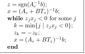
(vi) for eachB with |B| ≤∆ and for eachb ∈Rn the algorithm (Fig. 4.1) does
z= sgn(A−1
c b);
x= (Ac+BTz)−1b;
whilezjxj<0 for som ej
k= m in{j|zjxj <0};
zk=−zk;
x= (Ac+BTz)−1b;
[image:3.612.187.328.380.471.2]end
Fig. 4.1. The kernel of the sign accord algorithm.
not break down1
and in a finite number of steps (at most2n) yields the unique
solution of the equation
Acx+B|x|=b,
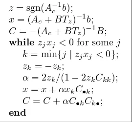
(vii) for each B with |B| ≤ ∆ and for each b ∈ Rn the sign accord algorithm
(Fig. 4.2) does not break down2
and in a finite number of steps (at most2n)
yields the unique solution of the equation
Acx+B|x|=b,
1
I.e., all the inverses exist. 2
z= sgn(A−1
c b);
x= (Ac+BTz)−1b;
C=−(Ac+BTz)−1B;
whilezjxj<0 for som ej
k= m in{j|zjxj<0};
zk=−zk;
α= 2zk/(1−2zkCkk);
x=x+αxkC•k;
C=C+αC•kCk•;
[image:4.612.189.324.104.229.2]end
Fig. 4.2.The sign accord algorithm.
(viii) for eachy∈Yn the equation
Acx−Ty∆|x|=y (4.3)
has a solution,
(ix) for eachy∈Yn the equation
Acx−Ty∆|x|=y
has a unique solution,
(x) for eachb >0 and for eachy∈Yn the equation
|Acx|= ∆|x|+b (4.4)
has a solutionxy satisfying Acxy∈Rny,
(xi) for eachb >0 and for eachy∈Yn the equation
|Acx|= ∆|x|+b
has a unique solutionxy satisfying Acxy∈Rny,
(xii) for eachy∈Yn the equation
|Acx|= ∆|x|+e
has a solutionxy satisfying Acxy∈Rny,
(xiii) for eachy∈Yn the equation
|Acx|= ∆|x|+e
has a unique solutionxy satisfying Acxy∈Rny,
(xiv) for eachy∈Yn the inequality
|Acx|>∆|x|
(xv) Ac is nonsingular and for eachb >0 the equation
|x|= ∆|A−1
c x|+b (4.5)
has a solution in each orthant,
(xvi) Ac is nonsingular and for eachb >0 the equation
|x|= ∆|A−1
c x|+b
has a unique solution in each orthant, (xvii) Ac is nonsingular and the equation
|x|= ∆|A−1
c x|+e
has a solution in each orthant, (xviii) Ac is nonsingular and the equation
|x|= ∆|A−1
c x|+e
has a unique solution in each orthant, (xix) Ac is nonsingular and the inequality
|x|>∆|A−1
c x| (4.6)
has a solution in each orthant,
(xx) there exists anR∈Rn×n such that the inequality
|x|>|(I−AcR)x|+ ∆|Rx| (4.7)
has a solution in each orthant, (xxi) for eachy∈Yn the matrix equation
AcX−Ty∆|X|=I (4.8)
has a solution,
(xxii) for eachy∈Yn the matrix equation
AcX−Ty∆|X|=I
has a unique solutionXy,
(xxiii) for eachy∈Yn the matrix equation
QAc− |Q|∆Ty =I (4.9)
has a solution,
(xxiv) for eachy∈Yn the matrix equation
QAc− |Q|∆Ty =I
(xxv) for eachy∈Yn the linear system
Ayex1−A−yex2=y, x1≥0, x2≥0
has a solution,
(xxvi) for eachy∈Yn,Aye is nonsingular and the system
A−1yeA−yex >0,
x >0
has a solution,
(xxvii) for eachy∈Yn,Aye andA−ye are nonsingular and the system
A−1yex >0,
A−1−yex >0
has a solution,
(xxviii) Ac is nonsingular and for eachy∈Yn,Aye is nonsingular and the system
|A−1
c Ty∆x|< x (4.10)
has a solution,
(xxix) for eachy∈Yn,Aye is nonsingular andA−1yeA−ye is aP-matrix,
(xxx) for eachy, z∈Yn,Ayz is nonsingular and
(AcA
−1
yz)ii>
1 2
holds for each i∈ {1, . . . , n},
(xxxi) det(Ac) det(Ayz)>0 for eachy, z∈Yn,
(xxxii) det(Ayz) det(Ay′z′)>0 for each y, z, y′, z′∈Yn,
(xxxiii) det(Ayz) det(Ay′z) > 0 for each y, y′, z ∈ Yn such that y and y′ differ in
exactly one entry, (xxxiv) Ac is nonsingular and
max
y,z∈Yn̺0(A
−1
c Ty∆Tz)<1
holds,
(xxxv) for each intervaln-vector bthe set
X(A,b) ={x|Ax=b for someA∈A, b∈b} (4.11)
is compact and connected,
(xxxvi) there exists an intervaln-vectorbfor which at least one component of the set X(A,b) ={x|Ax=b for someA∈A, b∈b}
(xxxvii) for eachx1, x2∈Rn,x1=x2, there holds
{Ax1|A∈A}{Ax2|A∈A}, (4.12)
(xxxviii) each matrix of the form
A=Ac−dTy∆Tz, (4.13)
whered∈[0,1]andy, z∈Yn, is nonsingular,
(xxxix) each matrix of the form
A=Ac−Tt∆Tz, (4.14)
where|t| ≤eandz∈Yn, is nonsingular,
(xl) each matrix of the form
Aij =
(Ayz)ij if eitheri=k, or i=kandj∈ {1, . . . , m−1},
(A−yz)ij ifi=kandj ∈ {m+ 1, . . . , n},
Akm ∈[Akm, Akm],
wherey, z∈Yn andk, m∈ {1, . . . , n}, is nonsingular,
(xli) each matrix of the form
Aij ∈
{Aij, Aij} if (i, j)= (k, m),
[Aij, Aij] if (i, j) = (k, m)
(i, j= 1, . . . , n), (4.15)
wherek, m∈ {1, . . . , n}, is nonsingular.
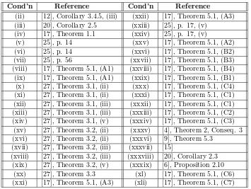
5. Sources. We do not give here the proof of the mutual equivalence of all the conditions since, as the reader may expect, this would make for a lengthy and perhaps tedious paper. Instead, we list in Fig. 5.1 a full list of their sources.
6. Comments. In this section we comment on the conditions. At some places we quote related theorems; for the sake of smoothness of the exposition, they are not marked as such, but are always given in italics. The forty conditions can be divided into five groups: (ii)-(vii), (viii)-(xxiv), (xxv)-(xxxiv), (xxxv)-(xxxvii), and (xxxviii)-(xli).
6.1. Conditions (ii)-(vii). The conditions (ii)-(vii) sumup the basic theoreti-cal and algorithmic facts.
(ii): This is the most important characterization, used in proofs of many other conditions. It is advantageous to read it negated: A is singular if and only if the inequality (4.1) has a nontrivial solution. If x = 0 solves (4.1), then a singular matrix S ∈A can be constructed as S =Ac−Ty∆Tz, where z = sgn(x) and y is
defined by yi = (Acx)i/(∆|x|)i if (∆|x|)i > 0 and yi = 1 otherwise, i = 1, . . . , n
([6], Proposition 2.10). In particular, (ii) gives that maxj(|A−1c |∆)jj ≥ 1 implies
Cond’n Reference Cond’n Reference
(ii) [12], Corollary 3.4.5, (iii) (xxii) [17], Theorem5.1, (A3) (iii) [20], Corollary 2.5 (xxiii) [25], p. 17, (v)
(iv) [17], Theorem1.1 (xxiv) [25], p. 17, (v)
(v) [25], p. 14 (xxv) [17], Theorem5.1, (A2) (vi) [25], p. 14 (xxvi) [17], Theorem5.1, (B2) (vii) [25], p. 56 (xxvii) [17], Theorem5.1, (B3) (viii) [17], Theorem5.1, (A1) (xxviii) [17], Theorem5.1, (B4) (ix) [17], Theorem5.1, (A1) (xxix) [17], Theorem5.1, (B1) (x) [27], Theorem3.1, (ii) (xxx) [17], Theorem5.1, (C4) (xi) [27], Theorem3.1, (ii) (xxxi) [17], Theorem5.1, (C1) (xii) [27], Theorem3.1, (iii) (xxxii) [17], Theorem5.1, (C1) (xiii) [27], Theorem3.1, (iii) (xxxiii) [17], Theorem5.1, (C2) (xiv) [27], Theorem3.1, (v) (xxxiv) [17], Theorem5.1, (C3)
(xv) [27], Theorem3.2, (ii) (xxxv) [4], Theorem2, Conseq. 3 (xvi) [27], Theorem3.2, (ii) (xxxvi) [9], Theorem5.3
(xvii) [27], Theorem3.2, (iii) (xxxvii) [15]
(xviii) [27], Theorem3.2, (iii) (xxxviii) [20], Corollary 2.3 (xix) [27], Theorem3.2, (v) (xxxix) [6], Proposition 2.10
[image:8.612.80.435.100.367.2](xx) [27], Theorem3.3 (xl) [17], Theorem5.1, (C6) (xxi) [17], Theorem5.1, (A3) (xli) [17], Theorem5.1, (C7)
Fig. 5.1.Sources of the conditions.
(xxxiv) below). Moreover, the condition (ii) is the main tool for the proof of co-NP-completeness of checking regularity (checking regularity of interval matrices of the form [Ac−eeT, Ac+eeT] is co-NP-complete in the class of nonnegative symmetric
positive definite rational matricesAc; short proof in [6], Theorem2.33, original proof
in [14]). This complexity result sheds its light on all the subsequent conditions: if the conjecture P=NP is true, then none of them is verifiable in polynomial time.
(iii): This condition shows that if (4.1) holds for somex= 0, then it also holds “uniformly” for some x′
= 0. It has a nontrivial consequence. Let us define a nonnegative number d to be an absolute eigenvalue of a real matrix A ∈ Rn×n if
|Ax|=d|x|holds for some realx= 0. Surprisingly enough,each square real matrix has an absolute eigenvalue([24], Theorem 5). Even more, the smallest absolute eigenvalue dmincan be given explicitly bydmin= inf{ε≥0|[A−εI, A+εI] is singular}([20], Theorem2.2).
(iv): This is a lemma-type assertion: it is of little use as such, but it is indis-pensable for the proofs of the subsequent important conditions (v) and (vi). In fact, Theorem1.1 in [17] states only necessity of (iv). But sufficiency follows easily by contradiction: if A is singular, then A′
x′
= 0 for som e A′
∈ A and x′
= 0, hence A′
x′ =A′
x′′
= 0 forx′′
= 0, butx′
jx
′′
j = 0 for eachj, a contradiction.
thereby enabling us to establish existence of certain uniquely defined objects (as the matricesXy, Qy in conditions (xxii), (xxiv), etc.).
(vi): The algorithmuses a while loop which is finite under the regularity as-sumption, although this is not obvious fromthe algorithmdescription (theoretically, it could return to the same z,xand cycle infinitely; in fact, this can appear ifA is singular ([17], Example 5.4)). Finiteness is proved by a sophisticated combinatorial argument based on condition (iv) (cycling would imply singularity). When the algo-rithmterminates in a finite number of steps, it is not difficult to see that the resulting xis a solution of (4.2), and its uniqueness follows fromthe condition (ii); this gives a constructive proof of (v).
(vii): The algorithmin condition (vi) requires explicit computation ofx= (A+ BTz)−1b at each step. In condition (vii), a Sherman-Morrison rank-one update is
used for this purpose; the updated values always satisfy x = (A+BTz)−1b, C =
−(A+BTz)−1B for the currentz. We present the algorithmin both forms because
the simple, although less effective form in (vi) better reveals its basic sign-accord-oriented mechanism (z, xare said to be in sign accord if they satisfy zjxj ≥0 for
eachj).
Comparison of (v) and (ii) gives rise to thefirst theorem of alternatives for real (noninterval) data ([24], Thms. 1 and 2): for each A, B ∈Rn×n, exactly one of the
alternatives (a), (b) holds: (a) For each B′
with|B′
| ≤ |B| and for each b∈Rn the
equation Ax+B′
|x| =b has a unique solution, (b) the inequality |Ax| ≤ |B||x| has a nontrivial solution. Here, (a) corresponds to regularity and (b) to singularity of [A− |B|, A+|B|].
6.2. Conditions (viii)-(xxiv). Conditions (viii)-(xxiv) concern equations and inequalities containing absolute values.
(viii)-(ix): The main contribution here consists in the fact that solvability of finitely many equations (4.3) implies unique solvability of infinitely many equations of the form(4.2). Notice that (viii) and (ix) differ only in the word “unique”. The same holds for several subsequent pairs of conditions ((x) and (xi), (xii) and (xiii), etc.).
(x)-(xiv): The strongest assertion here is (xi) which shows that for eachb >0 the set {Acx| |Acx| = ∆|x|+b} intersects all the orthants. The weakest one is (xiv),
and the proof of “(xiv)⇒(i)” [27] requires use of a little known existence theoremfor linear equations [18].
(xv)-(xx): (xv)-(xix) are counterparts of (x)-(xiv) formed by replacing the equa-tion (4.4) by (4.5). This results inunique solvability in each orthant, which is certainly a valuable property. The additional condition (xx) shows that the inequality (4.6) can be replaced by (4.7), thereby escaping the use of the exact inverseA−1
c . This is
a single example of using an approximate inverse among all the forty conditions. (xxi)-(xxii): For a regular interval matrixA, its inverse interval matrix is defined as A−1
= [B, B], where B = m in{A−1
|A ∈A}, B = m ax{A−1
| A∈ A} (com-ponentwise). Theorem6.2 in [17] asserts that the bounds of A−1 can be expressed by finite means asB = m iny∈YnXy,B= m axy∈YnXy (componentwise), whereXy is
(xxiii)-(xxiv): These conditions follow from(xxi), (xxii) when applied to the transpose interval matrixAT ={AT |A∈A}= [AT
c −∆T, ATc + ∆T]. The matrices
Qy, y ∈ Yn are used in the VERINTERVALHULL.M function [1] of VERSOFT [3]
for computing a verified interval hull of the solution set of interval linear equations (based on [25], Sections 4.3 and 7.11).
Comparison of (xi) and (ii) gives rise to thesecond theorem of alternatives (un-published): for each A, B ∈Rn×n, exactly one of the alternatives (a), (b) holds: (a)
For each b > 0 and for each orthant O of Rn the equation |Ax| − |B||x| = b has
a unique solution xO satisfying AxO ∈ O, (b) the equation |Ax| − |B||x| =b has a nontrivial solution for some b ≤ 0. Here, (a) corresponds to regularity and (b) to singularity of [A− |B|, A+|B|].
Comparison of (xiv) and (ii) gives rise to the third theorem of alternatives([27], Thm. 4.1): for each A, B ∈Rn×n, exactly one of the alternatives (a), (b) holds: (a)
For each orthant O of Rn the inequality |Ax| >|B||x| has a solution xO satisfying
AxO ∈ O, (b) the inequality |Ax| ≤ |B||x| has a nontrivial solution. Again, (a) corresponds to regularity and (b) to singularity of [A− |B|, A+|B|].
6.3. Conditions (xxv)-(xxxiv). Conditions (xxv)-(xxxiv) concern equations, inequalities and other expressions not containing absolute values3
.
(xxv): This condition is formulated in terms of n×2n linear systems. It is mainly a “return implication” used as the last member in a chain of implications (i)⇒(ii)⇒. . .⇒(ix)⇒(xxv)⇒(i). For a related more general result, see [23].
(xxvi)-(xxviii): The characteristic feature of these three conditions is their use of strict inequalities. They are seemingly of theoretical interest only; no application of themis known to the author so far.
(xxix): This condition brings about relationship between regularity and P -ma-trices (by definition, a square matrix is called a P-matrix if all its principal minors are positive). A general result published in [17], Thm. 1.2 says thatif A is regular, then A−11 A2 is a P-matrix for each A1, A2 ∈ A. Here it is shown that, conversely, the P-property of finitely many matrices of the formA−1
yeA−ye, y ∈ Yn, suffices to
enforce regularity.
(xxx): This is an example of using a finite set of inverses for checking regularity. It is used in S. M. Rump’s INTLAB function PLOTLINSOL.M [30] for verifying regularity of 2×2 interval matrices. As a necessary condition, it can be generalized:
if A is regular, then (AcA
−1 )ii >
1
2 for each A ∈ A and each i ∈ {1, . . . , n} ([17], Thm. 5.1, (C5)). The generalization to an arbitraryAis possible due to the inverse matrix representation theorem ([21], Thm. 1.1): ifAis regular, then for eachA∈A there exist nonnegative diagonal matrices Lyz, y, z∈Yn, satisfying Σy,z∈YnLyz =I
such that A−1
= Σy,z∈YnA−1yzLyz holds(a “convex combination”).
(xxxi)-(xxxii): Both the conditions say thatAis regular if and only if the deter-minants of all the matricesAyz, y, z ∈ Yn, are nonzero and of the same sign. The
sole nonsingularity of all the matrices Ayz, y, z∈ Yn, is not sufficient to guarantee
3
The inequality (4.10) in condition (xxviii) can be written without the absolute value as−x < A−c1T
regularity: a counterexample is given by the interval matrixA= [−I, I] which is sin-gular (it contains the zero matrix) despite nonsinsin-gularity of all theAyz’s (eachAyz is
a ±1-diagonal matrix). Condition (xxxi), due to its simplicity, can be recommended for solving classroom examples of small sizes.
(xxxiii): This is an equivalent, but more specific form of (xxxii). It is used in the proofs of conditions (xxx) and (xl).
(xxxiv): There are several applications of this condition. First, the radius of regularity defined by d(A) = inf{ε≥0 ; [Ac−ε∆, Ac+ε∆] is singular} can be
ex-pressed by finite means as d(A) = 1/maxy,z∈Yn̺0(A−1c Ty∆Tz) (Poljak and Rohn
[14]). Second, since̺0(A−1
c Ty∆Tz)≤̺(A−1c Ty∆Tz)≤̺(|A−1c Ty∆Tz|)≤̺(|A−1c |∆),
the condition̺(|A−1
c |∆) <1 implies regularity of A (originally proved by Beeck [5]
by simpler means). This is the most often used sufficient regularity condition (the so-called strong regularity); for complexity or verifiability purposes it can also be stated in an equivalent form(I− |A−1
c |∆)
−1≥0. Another sufficient regularity
condi-tion,σmax(∆)< σmin(Ac) (singular values), is due to Rump [29]; it follows from (ii).
Third, the condition (xxxiv) shows that an interval matrix of the form [I−∆, I+ ∆] is regular if and only if ̺(∆) <1, cf., [19]. And fourth, it implies that an interval matrix of the form [Ac−pqT, Ac+pqT], wherep, qare nonnegative column vectors in
Rn, is regular if and only ifT
qA−1c Tp∞,1<1 ([17], Thm . 5.2, (R2); see [22] for the norm · ∞,1). Finally, closely related to the condition (xxxiv) is the following result ([17], Thm. 4.6): ifTzA
−1
yzTy ≥0 and TzA
−1
−yzTy ≥0 for som ey, z∈ Yn, thenA is
regular and, moreover, TzA−1Ty ≥0 for each A∈ A. In particular, for y =z =e
we obtain that if A−1 ≥ 0 and A−1 ≥ 0, then A is regular and A−1
≥ 0 for each A∈A(Kuttler [11]); moreover, in this caseA−1
can be expanded into infinite series asA−1
= (∞
j=0(A
−1
(A−A))j)A−1 ([16], Thm. 2).
6.4. Conditions (xxxv)-(xxxvii). The next three conditions are formulated in terms of properties of certain sets.
(xxxv): The set (4.11) is called the solution set of a systemof interval linear equationsAx=b; it is described by the Oettli-Prager theorem[13] asX(A,b) ={x| |Acx−bc| ≤∆|x|+δ}(see [6], Thm. 2.9). The present condition makes it possible to
define the interval hullx(A,b) ofX(A,b) byx(A,b) = [minX(A,b), maxX(A,b)] (componentwise), i.e., as the narrowest interval vector containing it. In [25], p. 38, it is shown that using the matrices Qy fromcondition (xxiv), the interval hull can be
described explicitly byx(A,b) = [miny∈Yn(Qybc− |Qy|δ),maxy∈Yn(Qybc+|Qy|δ)],
(componentwise), whereb= [bc−δ, bc+δ]. Computing the interval hull is NP-hard
[28], therefore the problemof solving interval linear equations is often formulated as that of finding an interval vector x (not necessarily the optimal one) containing
X(A,b); such an interval vector is called an enclosure ofX(A,b). This, however, cannot be seen a universal recipe as an enclosure may essentially overestimate the interval hull, see, e.g., [26].
unbounded. Therefore, it suffices to enclose a single component ofX(A,b) to get an enclosure of the whole ofX(A,b) and simultaneously to prove regularity ofA. Both known not-a-priori-exponential algorithms for checking regularity [9], [2] employ this idea. The VERSOFT [3] function VERREGSING.M [2], moreover, yields verified
regularity or singularity.
(xxxvii): This condition was conjectured by K. RosNlaniec and proved in [15]. Indeed, the inclusion in (4.12) implies thatx1−x2 solves (4.1) and thus brings sin-gularity.
6.5. Conditions (xxxviii)-(xli). The last four conditions are best understood when negated: then they show that a singular interval matrix A contains singular matrices of several specific forms.
(xxxviii): This condition has a geometric interpretation: if A is singular, then it contains a singular matrix A = Ac−dTy∆Tz = (1−d)Ac +d(Ac −Ty∆Tz) =
(1−d)Ac +dAyz which belongs to the segment in Rn×n connecting the midpoint
matrixAc with a vertex matrixAyz.
(xxxix): A singular matrix of this form is returned in case of singularity by the VERSOFT [3] function VERREGSING.M [2]. It is constructed there froma nonzero solution of the inequality (4.1), see the construction ofS in the above comment on condition (ii).
(xl): This condition is most specific, but also most difficult to formulate, and seems to be the least used of the four.
(xli): Here again, we have a geometric interpretation: if A is singular, then it contains a singular matrix belonging to an edge ofAwhen considered a rectangle in theRn2
space. An eigenvalue version of this “edge theorem” was given in [10], Thm. 21.21, and a more general result was achieved by Hollot and Bartlett [7].
Acknowledgment. The author thanks the referee for comments that helped improve the text of this paper.
REFERENCES
[1] VERINTERVALHULL: Verified interval hull of the solution set of a system of interval linear equations, 2007. Available at http://www.cs.cas.cz/rohn/matlab/verintervalhull.html.
[2] VERREGSING: Verified regularity/singularity of an interval matrix, 2007. Available at
http://www.cs.cas.cz/rohn/matlab/verregsing.html.
[3] VERSOFT: Verification software in MATLAB/INTLAB, 2009. Available at
http://www.cs.cas.cz/rohn/matlab.
[4] H. Beeck. Charakterisierung der L¨osungsmenge von Intervallgleichungssystemen. Zeitschrift f¨ur Angewandte Mathematik und Mechanik, 53:T181–T182, 1973.
[5] H. Beeck. Zur Problematik der H¨ullenbestimmung von Intervallgleichungssystemen. In
K. Nickel, editor,Interval Mathematics, Lecture Notes in Computer Science 29, pp. 150– 159, Berlin, 1975. Springer-Verlag.
[6] M. Fiedler, J. Nedoma, J. Ram´ık, J. Rohn, and K. Zimmermann.Linear Optimization Problems with Inexact Data. Springer-Verlag, New York, 2006.
[7] C. V. Hollot and A. C. Bartlett. On the eigenvalues of interval matrices. Proceedings of the 26th Conference on Decision and Control, Los Angeles, CA, pp. 794–799, 1987.
[9] C. Jansson and J. Rohn. An algorithm for checking regularity of interval matrices. SIAM Journal on Matrix Analysis and Applications, 20:756–776, 1999.
[10] V. Kreinovich, A. Lakeyev, J. Rohn, and P. Kahl. Computational Complexity and Feasibility of Data Processing and Interval Computations. Kluwer Academic Publishers, Dordrecht, 1998.
[11] J. Kuttler. Afourth-order finite-difference approximation for the fixed membrane eigenproblem.
Mathematics of Computation, 25:237–256, 1971.
[12] A. Neumaier. Interval Methods for Systems of Equations. Cambridge University Press, Cam-bridge, 1990.
[13] W. Oettli and W. Prager. Compatibility of approximate solution of linear equations with given error bounds for coefficients and right-hand sides. Numerische Mathematik, 6:405–409, 1964.
[14] S. Poljak and J. Rohn. Checking robust nonsingularity is NP-hard. Mathematics of Control, Signals, and Systems, 6:1–9, 1993.
[15] J. Rohn. Solution of a problem proposed by K. RosOlaniec on March 12, 1999. Submission to thereliable computingnet of March 15, 1999.
[16] J. Rohn. Inverse-positive interval matrices. Zeitschrift f¨ur Angewandte Mathematik und Mechanik, 67:T492–T493, 1987.
[17] J. Rohn. Systems of linear interval equations. Linear Algebra and its Applications, 126:39–78, 1989.
[18] J. Rohn. An existence theorem for systems of linear equations.Linear and Multilinear Algebra, 29:141–144, 1991.
[19] J. Rohn. Cheap and tight bounds: The recent result by E. Hansen can be made more efficient.
Interval Computations, 4:13–21, 1993.
[20] J. Rohn. Interval matrices: Singularity and real eigenvalues.SIAM Journal on Matrix Analysis and Applications, 14:82–91, 1993.
[21] J. Rohn. Inverse interval matrix. SIAM Journal on Numerical Analysis, 30:864–870, 1993. [22] J. Rohn. Computing the normA∞
,1is NP-hard.Linear and Multilinear Algebra, 47:195–204, 2000.
[23] J. Rohn. Solvability of systems of linear interval equations. SIAM Journal on Matrix Analysis and Applications, 25:237–245, 2003.
[24] J. Rohn. Atheorem of the alternatives for the equationAx+B|x|=b.Linear and Multilinear Algebra, 52:421–426, 2004.
[25] J. Rohn. Ahandbook of results on interval linear problems, 2005. Internet text available at http://www.cs.cas.cz/rohn/handbook.
[26] J. Rohn. Linear interval equations: Midpoint preconditioning may produce a 100% overesti-mation for arbitrarily narrow data even in casen= 4. Reliable Computing, 11:129–135, 2005.
[27] J. Rohn. Regularity of interval matrices and theorems of the alternatives. Reliable Computing, 12:99–105, 2006.
[28] J. Rohn and V. Kreinovich. Computing exact componentwise bounds on solutions of linear systems with interval data is NP-hard.SIAM Journal on Matrix Analysis and Applications, 16:415–420, 1995.
[29] S. M. Rump. Verification methods for dense and sparse systems of equations. In J. Herzberger, editor,Topics in Validated Computations, pages 63–135, Amsterdam, 1994. North-Holland.
[30] S. M. Rump. INTLAB - INTerval LABoratory, 2009. Available at