El e c t ro n ic
Jo ur n
a l o
f P
r o b
a b i l i t y
Vol. 13 (2008), Paper no. 27, pages 852–879. Journal URL
http://www.math.washington.edu/~ejpecp/
Malliavin Calculus in L´
evy spaces and Applications
to Finance
Evangelia Petrou∗
Institut f¨ur Mathematik, Technische Universit¨at Berlin
Abstract
The main goal of this paper is to generalize the results of Fourni´e et al. [8] for markets generated by L´evy processes. For this reason we extend the theory of Malliavin calculus to provide the tools that are necessary for the calculation of the sensitivities, such as differen-tiability results for the solution of a stochastic differential equation .
Key words: L´evy processes, Malliavin Calculus, Monte Carlo methods, Greeks. AMS 2000 Subject Classification: Primary 60H07, 60G5.
Submitted to EJP on June 5, 2007, final version accepted April 7, 2008.
1
Introduction
In recent years there has been an increasing interest in Malliavin Calculus and its applications to finance. Such applications were first presented in the seminal paper of Fourni´e et al. [8]. In this paper the authors are able to calculate the Greeks using well known results of Malliavin Calculus on Wiener spaces, such as the chain rule and the integration by parts formula. Their method produces better convergence results from other established methods, especially for discontinuous payoff functions.
There have been a number of papers trying to produce similar results for markets generated by pure jump and jump-diffusion processes. For instance El-Khatib and Privault [6] have consid-ered a market generated by Poisson processes. In Forster et al. [7] the authors work in a space generated by independent Wiener and Poisson processes; by conditioning on the jump part, they are able to calculate the Greeks using classical Malliavin calculus. Davis and Johansson [4] produce the Greeks for simple jump-diffusion processes which satisfy a separability condition. Each of the previous approaches has its advantages in specific cases. However, they can only treat subgroups of L´evy processes.
This paper produces a global treatment for markets generated by L´evy processes and achieves a similar formulation of the sensitivities as in Fourni´e et al. [8]. We rely on Malliavin calculus for discontinuous processes and expand the theory to fulfill our needs. Malliavin calculus for dis-continuous processes has been widely studied as an individual subject, see for instance Bichteler et al. [3] for an overview of early works, Di Nunno et al. [5], Løkka [12] and Nualart and Vives [14] for pure jump L´evy processes, Sol´e et al. [16] for general L´evy processes and Yablonski [17] for processes with independent increments. It has also been studied in the sphere of finance, see for instance Benth et al. [2] and L´eon et al. [11]. In our case we focus on square integrable L´evy processes.
The starting point of our approach is the fact that L´evy processes can be decomposed into a Wiener process and a Poisson random measure part. Hence we are able to use the results of Itˆo [9] on the chaos expansion property. In this way every square integrable random variable in our space can be represented as an infinite sum of integrals with respect to the Wiener process and the Poisson random measure. Having the chaos expansion we are able to introduce operators for the Wiener processes and Poisson random measure. With an application to finance in mind, the Wiener operator should preserve the chain rule property. Such a Wiener operator was introduced in Yablonski [17] for the more general class of processes with independent increments, using the classical Malliavin definition. In our case we adopt the definition of directional derivative first introduced in Nualart and Vives [14] for pure jump processes and then used in L´eon et al. [11] and Sol´e et al.[16]. The chain rule formulation that is achieved for simple L´evy processes in L´eon et al. [11], and for more general processes in Sol´e et al. [16], is only applicable to separable random variables. As Davis and Johansson [4] have shown, this form of chain rule restricts the scope of applications, for instance it excludes stochastic volatility models that allow jumps in the volatility. We are able to bypass the separability condition, by generalizing the chain rule in this setting. Following this, we define the directional Skorohod integrals, conduct a study of their properties and give a proof of the integration by parts formula. We conclude our theoretical part with the main result of the paper, the study of differentiability for the solution of a L´evy stochastic differential equation.
The paper is organized as follows. In Section 2 we summarize results of Malliavin calculus, de-fine the two directional derivatives, in the Wiener and Poison random measure direction, prove their equivalence to the classical Malliavin derivative and the difference operator in Løkka [12] respectively, and prove the general chain rule. In Section 3 we define the adjoint of the direc-tional derivatives, the Skorohod integrals, and prove an integration by parts formula. In Section 4 we prove the differentiability of a solution of a L´evy stochastic differential equation and get an explicit form for the Wiener directional derivative. Section 5 deals with the calculation of the sensitivities using these results. The paper concludes in Section 6, with the implementation of the results and some numerical experiments.
2
Malliavin calculus for square integrable L´
evy Processes
LetZ ={Zt, t∈[0, T]}be a centered square integrable L´evy process on a complete probability
space (Ω,F,{Ft}t∈[0,T],P), where {Ft}0≤t≤T is the augmented filtration generated byZ. Then
the process can be represented as:
Zt=σWt+
Z t
0
Z
R0
z(µ−π)(dz, ds)
where{Wt}t∈[0,T] is the standard Wiener process andµ(·,·) is a Poisson random measure inde-pendent of the Wiener process defined by
µ(A, t) =X
s≤t
1A(∆Zs)
whereA∈ B(R0) . The compensator of the L´evy measure is denoted by π(dz, dt) =λ(dt)ν(dz) and the jump measure of the L´evy process by ν(·), for more details see [1]. Since Z is square integrable the L´evy measure satisfies R
R0z
2ν(dz) < ∞. Finally σ is a positive constant, λthe Lebesgue measure and R0 = R\ {0}. In the following ˜µ(ds, dz) = µ(ds, dz)−π(ds, dz) will represent the compensated random measure.
In order to simplify the presentation, we introduce the following unifying notation for the Wiener process and the random Poisson measure
U0 = [0, T] and U1= [0, T]×R
dQ0(·) =dW· and Q1= ˜µ(·,·)
dhQ0i=dλ and dhQ1i=dλ×dν
ulk =
tk , l= 0
(tk, x), l= 1.
also we define an expanded simplex of the form:
Gj1,...,jn =
(
(uj1
1 , . . . , ujnn)∈ n
Y
i=1
Uji : 0< t1 <· · ·< tn< T
) ,
forj1, . . . , jn= 0,1.
Finally, J(j1,...,jn)
n (gj1,...,jn) will denote the (n-fold) iterated integral of the form
J(j1,...,jn)
n (gj1,...,jn) =
Z
Gj1,...,jn
gj1,...,jn(u j1
1, . . . , ujnn)Qj1(duj11). . . Qjn(du jn
wheregj1,...,jn is a deterministic function inL
2(G
j1,...,jn) =L
2(G
j1,...,jn,
Nn
i=1dhQjii).
2.1 Chaos expansion
The theorem that follows is the chaos expansion for processes in the L´evy spaceL2(Ω). It states that every random variable F in this space can be uniquely represented as an infinite sum of integrals of the form (1). This can be considered as a reformulation of the results in [9], or an expansion of the results in [12].
Theorem 1. For every random variable F ∈ L2(FT,P), there exists a unique sequence
{gj1,...,jn}∞n=0, j1, . . . , jn= 0,1, where gj1,...,jn ∈L
2(G
j1,...,jn) such that
F =
∞
X
n=0
X
j1,...,jn=0,1
J(j1,...,jn)
n (gj1,...,jn) (2)
and we have the isometry
kFk2L2(P) = ∞
X
n=0
X
j1,...,jn=0,1
kJ(j1,...,jn)
n (gj1,...,jn)k
2
L2(G
j1,...,jn).
2.1.1 Directional derivative
Given the chaos expansion we are able to define directional derivatives in the Wiener process and the Poisson random measure. For this we need to introduce the following modification to the expanded simplex
Gkj1,...,jn(t) = n(uj1
1 , . . . ,uˆ
jk
k , . . . , u jn
n)∈Gj1,...,jk−1,jk+1,...,jn :
0< t1<· · ·< tk−1 < t < tk+1· · ·< tn< T},
where ˆumeans that we omit theuelement. Note thatGkj1,...,jn(t)∩Glj1,...,jn(t) =∅ifk6=l. The definition of the directional derivatives follows the one in [11].
Definition 1. Let gj1,...,jn ∈L
2(G
j1,...,jn) and l= 0,1. Then
Du(ll)J
(j1,...,jn)
n (gj1,...,jn) =
n
X
i=1
1{ji=l}J
(j1,...,ˆji,...,jn)
n−1
gj1,...,jn(. . . , u
l, . . .)1 Gi
j1,...,jn(t)
is called the derivative of J(j1,...,jn)
n (gj1,...,jn) in the l-th direction.
We can show that this definition is reduced to the Malliavin derivative if we take
ji= 0,∀i= 1, . . . , n, and to the definition of [12] ifji = 1,∀i= 1, . . . , n.
Definition 2. 1. LetD(l) be the space of the random variables inL2(Ω)that are differentiable in the l-th direction, then
D(l) = {F ∈L2(Ω), F =E[F] +
∞
X
n=1
X
j1,...,jn=0,1
J(j1,...,jn)
n (gn) :
∞
X
n=1
X
j1,...,jn=0,1
n
X
i=1
1{ji=l}
Z
Ujik
gj1,...,jn(·, u
l,
·)k2L2(Gi i1,...,in)
×dhQli(ul)<∞}.
2. Let F ∈D(l). Then the derivative on the l-th direction is:
Du(ll)F =
∞
X
n=1
X
j1,...,jn=0,1
n
X
i=1
1{ji=l}J
(j1,...,ˆji,...,jn)
n−1
gj1,...,jn(·, u
l,
·)1Gi
j1,...,jn(t)
.
From the definition of the domain of thel−directional derivative, all the elements ofL2(Ω) with finite chaos expansion are included inD(l). Hence, we can conclude thatD(l) is dense inL2(Ω).
2.1.2 Relation between the Classical and the Directional Derivatives
In order to study the relation between the classical Malliavin derivative, see [13], the difference operator in [12] and the directional derivatives, we need to work on the canonical space. The canonical Brownian motion is defined on the probability space (ΩW,FW,PW), where ΩW =
C0([0,1]); the space of continuous functions on [0,1] equal to null at time zero; FW is the Borel
σ-algebra and PW is the probability measure on FW such that Bt(ω) := ω(t) is a Brownian
motion.
Respectively, the triplet (ΩN,FN,PN) denotes the space on which the canonical Poisson random
measure. We denote with ΩN the space of integer valued measures ω′ on [0,1]×R0, such that
ω′(t, u)≤1 for any point (t, u)∈[0,1]×R0, andω′(A×B)<∞whenπ(A×B) =λ(A)ν(B)<∞, whereν is theσ-finite measure on R0. The canonical random measure on ΩN is defined as
µ(ω′, A×B) :=ω′(A×B).
WithPN we denote the probability measure onFN under whichµis a Poisson random measure
with intensity π. Hence, µ(A×B) is a Poisson variable with meanπ(A×B), and the variables
µ(Ai×Bj) are independent when Ai×Bj are disjoint.
In our case we have a combination of the two above spaces. With (Ω,F,{Ft}t∈[0,1],P) we will denote the joint probability space,where
Ω := ΩW ⊗ΩN equipped with the probability measureP:=PW ⊗PN and Ft:=FtW ⊗ FtN.
Then there exists an isometry
L2(ΩW ×ΩN)≃L2(ΩW;L2(ΩN)),
where
L2(ΩW;L2(ΩN)) ={F : ΩW →L2(ΩN) :
Z
ΩW
kF(ω)k2L2(Ω
Therefore we can consider every F ∈ L2(ΩW;L2(ΩN)) as a functional F : ω → F(ω, ω′).
This implies that L2(ΩW;L2(ΩN)) is a Wiener space on which we can define the classical
Malliavin derivative D. The derivative D is a closed operator from L2(ΩW;L2(ΩN)) into
L2(ΩW ×[0,1];L2(ΩN)). We denote with D1,2 the domain of the classical Malliavin deriva-tive. IfF ∈D1,2, then
DF ∈ L2(ΩW;L2(ΩN;L2([0,1])))
≃ L2(ΩW ×ΩN ×[0,1])
In the same way the difference operator ˜D defined in [12] with domain ˜D1,2 is closed from
L2(ΩN;L2(ΩW)) intoL2(ΩN ×[0,1];L2(ΩW)). If F ∈D˜1,2, then
˜
DF ∈ L2(ΩN;L2(ΩW;L2([0,1])))
≃ L2(ΩN ×ΩW ×[0,1])
As a consequence we have the following proposition.
Proposition 1. On the space D(0) the directional derivative D(0) is equivalent to the classical Malliavin derivative D, i.e. D = D(0). Respectively on D(1) the directional derivative D(1) is equivalent the difference operator D˜, i.e. D˜ =D(1).
Given the directional derivatives Dand ˜Dwe reach the subsequent proposition.
Proposition 2. 1. LetF =f(Z, Z′)∈L2(Ω), whereZ depends only on the Wiener part and
Z ∈D(0), Z′ depends only on the Poisson random measure and f(x, y) is a continuously differentiable function with bounded partial derivatives in x, then
D(0)F = ∂
∂xf(Z, Z
′)D(0)Z
2. Let F ∈D(1) then
D(1)(t,z)F =F ◦ǫ+(t,z)−F,
where ǫ+ is a transformation on Ωgiven by
ǫ−(t,z)ω(A×B) =ω(A×B∩(t, z)c),
ǫ+(t,z)ω(A×B) =ǫ−(t,z)ω(A×B) +1A(t)1B(z).
2.1.3 Chain rule
The last proposition is an extension of the results in [11], where the authors consider only simple L´evy processes, and similar to corollary 3.6 in [16]. However, this chain rule is applicable to random variables that can be separated to a continuous and a discontinuous part;separable random variables, for more details see [4]. In what follows we provide the proof of chain rule with no separability requirements.
γ(z) =
Proof. The proof follows the same steps of [12].
The proof of the chain rule requires the next technical lemma.
Lemma 2. Let F ∈ D(0) and {Fk}∞k=1 be a sequence such that Fk ∈ D(0) and Fk → F in
Proof. We follow the same steps as in Lemma 6 in [12]. Since Fk converges to F
lim
Since Fk, F ∈D(0) from the definition of the directional derivative we have
From (4) we can choose a subsequence such that kgkm+1
j1,...,jn)= 0. From the dominate convergence theorem
we have
Using the fact that D(0) is a densely defined and closed operator, and that the elements of the linear span S are separable processes, we prove in the following theorem the chain rule for all processes in D(0).
Theorem 2. (Chain Rule) Let F ∈D(0) and f be a continuously differentiable function with bounded derivative. Thenf(F)∈D(0) and the following chain rule holds:
D(0)f(F) =f′(F)D(0)F. (5)
Remark.The theory developed in this chapter also holds in the case that our space is generated by and-dimensional Wiener process and k-dimensional random Poisson measures. However, we will have to introduce new notation for the directional derivatives in order to simplify things. For the multidimensional case,D(0)t F will denote a row vector, where the element of thei-th row is the directional derivative for the Wiener processWi , for all i= 1, . . . , d. Similarly we define
the row vectorD(1)(t,z)F. FurthermoreDiF ,i= 1, . . . , d, will be scalars denoting the directional derivative of the i-th Wiener process Wi fori= 1, . . . , d, and the derivative in the direction of thei-th random Poisson measure ˜µi fori=d+ 1, . . . , d+k.
3
Skorohod Integral
The next step after the definition of the directional derivatives is to define their adjoint, which are the Skorohod integrals in the Wiener and Poisson random measure directions.
The first two result of the section are the calculation of the Skorohod integral and the study of its relation to the Itˆo and Stieltjes-Lebesgue integrals. These are extensions of the results in [4] and [10] from simple Poisson processes to square integrable L´evy processes. The proof are performed in parallel ways as in [4] (or in more detail in [10]), therefore they are omitted. The main result however is an integration by parts formula. Although the separability result is yet again an extension of [4], having attained a chain rule for D(0) that does not require a condition, we are able to provide a simpler and more elegant proof. Finally the section closes with a technical result.
Definition 3. The Skorohod integral
Let δ(l) be the adjoint operator of the directional derivative D(l),l= 0,1. The operatorδ(l) maps
L2(Ω×Ul) to L2(Ω). The set of processes h∈L2(Ω×Ul) such that:
E
Z
Ul
(D(ul)F)htdhQli
≤ckFk, (6)
for allF ∈D(l), is the domain of δ(l), denoted by Domδ(l).
For everyh∈Domδ(l) we can define the Skorohod integral in the l-th directionδ(l)(h) for which
E Z
Ul
(D(ul)F)htdhQli
=E[F δ(l)(h)] (7)
for anyF ∈D(l).
The following proposition provides the form of the Skorohod integral.
Proposition 3. Forh(u)∈L2(Ul) and F ∈L2(Ω)with chaos expansion
F =E(F) +
∞
X
n=1
X
j1,...,jn=0,1
J(j1,...,jn)
Then the l-th directional Skorohod integral is
Having the exact form of the Skorohod integral we can study its properties. For instance the Skorohod integral can be reduced to an Itˆo or Stieltjes-Lebesgue integral in the case of predicable processes.
Proposition 4. Let ht be a predictable process such that E[
R
We are now able to prove one of the main results, the integration by parts formula.
Proposition 5. (Integration by parts formula) Let F h ∈L2(Ω×[0, T]), where F ∈D(0),
ht is predictable square integrable process. Then F h∈Domδ(0) and
δ(0)(F h) =F
Proof. From Theorem 2 we have
E
of the Skorohod integral we have
E[
Z T
0
Dt(0)G·F ·udt] =E[G·δ(0)(F·u)]. (9)
Combining (8), (9) and Proposition 4 the proof is concluded.
Note that when F is an m-dimensional vector process and h a m ×m matrix process the
integration by part formula can be written as follows:
δ(0)(F h) =F∗
Proposition 6. Let ht be a predictable square integrable process. Then
• if h∈D(0) then
D(0)t Z T
0
hsdWs=ht+
Z T
t
D(0)s hsdWs
Dt(0) Z T
0
Z
R0
hsµ˜(dz, ds) =
Z T
t
Z
R0
D(0)s hsµ˜(dz, ds)
• if h∈D(1) then
D(1)(t,z) Z T
0
hsdWs=
Z T
t
D(1)(s,z)hsdWs
D(1)(t,z) Z T
0
Z
R0
hsµ˜(dz, ds) =ht+
Z T
t
Z
R0
D((1)s,z)hsµ˜(dz, ds)
Proof. This result can be easily deduced from the definition of the directional derivative.
4
Differentiability of Stochastic Differential
Equations
The aim of this section is to prove that under specific conditions the solution of a stochastic differential equation belongs to the domains of the directional derivatives. Having in mind the applications in finance, we will also provide a specific expression for the Wiener directional derivative of the solution.
Let {Xt}t∈[0,T] be an m-dimensional process in our probability space, satisfying the following stochastic differential equation:
dXt = b(t, Xt−)dt+σ(t, Xt−)dWt+
Z
R0
γ(t, z, Xt−)˜µ(dz, dt)
X0 = x (10)
wherex∈Rm,{Wt}t∈[0,T]is ad-dimensional Wiener process, ˜µis a compensated Poisson random measure. The coefficients b: R×Rm → Rm,σ :R×Rm → Rm×Rd and γ :R×R×Rm → Rm×R, are continuously differentiable with bounded derivatives. The coefficients also satisfy
the following linear growth condition:
kb(t, x)k2+kσ(t, x)k2+
Z
R0
kγ(t, z, x)k2ν(dz)≤C(1 +kxk2),
for eacht∈[0, T], x∈Rm where C is a positive constant. Furthermore there exists ρ:R→R
withR
R0ρ(z)
2ν(dz)<∞, and a positive constantD such that
for all x, y∈Rm and z∈R0.
Under these conditions there exists a solution for (10) which is also unique1. For what follows we denote withσi thei-th column vector ofσ and adopt the Einstein convention of leaving the
summations implicit.
In the next theorem we prove that the solution{Xt}t∈[0,T]is differentiable in both directions of the Malliavin derivative. Moreover we reach the stochastic differentiable equations satisfied by the derivatives.
Theorem 3. Let {Xt}t∈[0,T] be the solution of (10). Then
1. Xt∈D(0),∀t∈[0, T]and the derivative Ds(i)Xt satisfies the following linear equation:
DisXt =
Z t
s
∂ ∂xk
b(r, Xr−)DsiXrk−dr
+ σi(s, Xs−) + Z t
s
∂ ∂xk
σα(r, Xr−)DisXrk−dW
α r
+
Z t
s
Z
R0 ∂ ∂xk
γ(r, z, Xr−)DsiXrk−µ˜(dz, dr) (12)
for s≤t a.e. and
DisXt= 0, a.e. otherwise.
2. Xt∈D(1),∀t∈[0, T]and the derivative D((1)s,z)Xt satisfies the following linear equation
D(1)(s,z)Xt =
Z t
s
D(1)(s,z)b(r, Xr−)dr
+
Z t
s
D(1)(s,z)σ(r, Xr−)dWr
+ γ(s, z, Xs−) + Z t
s
Z
R0
D((1)s,z)γ(r, z, Xr−)˜µ(dz, dr) (13)
for s≤t a.e., with
D(1)(s,z)Xt= 0, a.e. otherwise.
Proof. 1. Using Picard’s approximation scheme we introduce the following process
Xt0 = x0
Xtn+1 = x0+
Z t
0
b(s, Xsn−)ds+ Z t
0
σj(s, Xsn−)dW
j s
+
Z t
0
Z
R0
γ(s, z, Xsn−)˜µ(dz, ds) (14)
ifn≥0.
We prove by induction that the following hypothesis holds true for all n≥0. (H)Xtn∈D(0) for allt∈[0, T],
It is straightforward that (H) is satisfied for n = 0. Let us assume that (H) is satis-fied for n ≥ 0. Then from Theorem 2, b(s, Xn
Furthermore, we have that
D(0)r bj(s, Xsn−) =
Since the coefficients have continuously bounded first derivatives in the x direction and condition (11), there exists a constantK such that
|D(0)r bj(s, Xsn−)| ≤K|D(0)r Xsn−| (15)
(0) from Proposition 6. Thus,
From the above we can conclude thatXtn+1 ∈D(0) for allt∈[0, T]. Furthermore
From Cauchy-Schwartz and Burkholder-Davis-Gundy2 inequality, (19) takes the following form
Thus, hypothesis (H) holds for n+ 1. From Applebaum [1], Theorem 6.2.3, we have that
E sup
s≤T|
Xsn−Xs|2
!
→0
asngoes to infinity.
By induction to the inequality (20), see for more details appendix A, we can conclude that the derivatives of Xsn are bounded in L2(Ω×[0, T]) uniformly in n. Hence Xt ∈ D(0).
Applying the chain rule to (12) we conclude our proof.
2. Following the same steps we can prove the second claim of the theorem.
With the previous theorem we have proven that the solution of (10) is inD(0), and reached the
stochastic differential equation thatD(0)s Xtsatisfies. However, the Wiener directional derivative
can take a more explicit form. As in the classical Malliavin calculus we are able to associate the solution of (12) with the process Yt =∇Xt; first variation ofXt. Y satisfies the following
stochastic differential equation3:
dYt = b
′
(t, Xt−)Yt−dt+σ ′
i(t, Xt−)Yt−dWti
+
Z
R0
γ′(t, z, Xt−)Yt−µ˜(dz, dt)
Y0 = I, (21)
where prime denotes the derivative and I the identity matrix. Hence, we reach the following proposition which provides us with a simpler expression forD(0)s Xt.
Proposition 7. Let{Xt}t∈[0,T] be the solution of (10). Then the derivativeD(0)t in the Wiener
direction satisfies the following equation:
Dr(0)Xt=YtYr−−1σ(r, Xr−), ∀r ≤t, (22)
where Yt=∇Xt is the first variation of Xt.
Proof. The elements of the matrixY satisfy the following equation:
Ytij = δji+
Z t
0
∂ ∂xk
bi(s, Xs−)Yskjds
+
Z t
0
∂ ∂xα
σik(s, Xs−)YskjdWsα
+
Z t
0
Z
R0 ∂ ∂xk
γi(s, z, Xs−)Yskjµ˜(dz, ds),
whereδ is the Dirichlet delta.
Let{Zt}t∈[0,T]be a d×dmatrix valued process that satisfies the following equation
Ztij = δij+
Z t
0
−∂x∂
j
bk(t, Xs−) + ∂ ∂xl
σαk(t, Xs−) ∂ ∂xj
σlα(t, Xs−)
Zsik−ds
+
Z t
0
Z
R0
∂ ∂xkγ
i(t, z, X s−)
2
1 + ∂
∂xkγ
i(t, z, X s−)
Zsik−ν(dz)ds
−
Z t
0
∂ ∂xl
σkj(t, Xs−)Zsik−dW
l s
−
Z t
0
Z
R0
∂ ∂xkγ
i(t, z, X s−)
1 +∂x∂
kγ
i(t, z, X s−)
Zsik−µ˜(dz, ds)
By applying integration by parts formula we can prove that YtZt=ZtYt=I,
ZtijYtjl = δil
Hence, Zt = Yt−1. Furthermore it is easy to show applying again Itˆo’s formula, that
Yil
t Zrlk−σkj(r, Xr−) verifies (12) for all r < t. Hence the proof is concluded.
5
Sensitivities
Using the Malliavin calculus developed in the previous sections we are able to calculate the sensitivities, i.e. the Greek letters. The Greeks are calculated for an m-dimensional process {Xt}t∈[0,T]that satisfies equation (10).
We denote the price of the contingent claim as
u(x) =E[φ(Xt1, . . . , Xtn)], (23)
where φ(Xt1, . . . , Xtn) is the payoff function, which is square integrable, evaluated at times
t1, . . . , tn and discounted from maturityT.
In what follows we assume the following ellipticity condition for the diffusion matrixσ.
Assumption 1. The diffusion matrix σ is elliptic. That implies that there exists k > 0 such that
y∗σ∗(t, x)σ(t, x)y≥k|y|2, ∀y, x∈Rd.
5.1 Variation in the Drift Coefficient
Let us assume the following perturbed process
dXtǫ = b(t, Xtǫ−) +ǫξ(t, X
ǫ t−)
dt+σ(t, Xtǫ−)dWt
+
Z
R0
γ(t, z, Xtǫ−)˜µ(dz, dt),
X0 = x
Proposition 8. Let σ be a uniformly elliptic matrix. We denoteuǫ(x) the following payoff
uǫ(x) =E[φ(XTǫ)].
Then
∂uǫ(x)
∂ǫ
ǫ=0
=E[φ(XT)
Z T
0
(σ−1(t, Xt−)ξ(t, Xt−))∗dWt].
Proof. The proof is based on an application of Girsanov’s theorem. For
MT = exp (−ǫ
Z T
0
(σ−1(t, Xt−)ξ(Xt−))∗dWt)−
ǫ2
2
Z T
0 k
σ−1(t, Xt−)γ(Xt−)k2dt)
we have
E[φ(XTǫ)] =E[MTφ(XT)]
Hence
∂u(x)
∂ǫ
ǫ=0
= lim
ǫ→0E
hφ(Xǫ
T)−φ(XT)
ǫ
i
= lim
ǫ→0E
h φ(XT)
MTǫ −1
ǫ i
= Ehφ(XT)
Z T
0
(σ−1(t, Xt−)ξ(t, Xt−))∗dWt
i
5.2 Variation in the Initial Condition
In order to calculate the variation in the initial condition we will define the set Γ, as follows
Γ ={ζ ∈L2([0, T)) :
Z ti
0
ζ(t)dt= 1,∀i= 1, . . . , n}
whereti are as in (23).
Proposition 9. Assume that the diffusion matrix σ is uniformly elliptic. Then for all ζ(t)∈Γ
(▽u(x))∗ =Ehφ(Xt1, . . . , Xtn)
Z T
0
ζ(t)(σ−1(t, Xt−)Yt−)∗dWt
i
Proof. Let φ be a continuously differentiable function with bounded gradient. Then we can differentiate inside the expectation4 and we have
∇u(x) = E[
n
X
i=1
∇iφ(Xt1, . . . , Xtn)
∂ ∂xXti]
= E[
n
X
i=1
∇iφ(Xt1, . . . , Xtn)Yti], (24)
where∇iφ(Xt1, . . . , Xtn) is the gradient ofφwith respect toXti, and
∂
∂xXti is thed×dmatrix
of the first variation of the d-dimensional process Xti.
From (22) we have
Yti = D
(0)
t Xtiσ−
1(t, X
t−)Yt−.
Hence for anyζ ∈Γ
Yti =
Z T
0
ζ(t)Dt(0)Xtiσ−
1(t, X
t−)Yt−dt
and inserting the above to (24) follows that
∇u(x) =E[
Z T
0
n
X
i=1
∇iφ(Xt1, . . . , Xtn)ζ(t)D
(0)
t Xtiσ−
1(t, X
t−)Yt−dt]
from Theorem 2φ(Xt1, . . . , Xtn)∈D
(0), thus
∇u(x) = E[
Z T
0
Dt(0)φ(Xt1, . . . , Xtn)ζ(t)σ−
1(t, X
t−)Yt−dt]
From the definition of the Skorohod integral we reach
(∇u(x))∗ = E[φ(Xt1, . . . , Xtn)δ
(0) ζ(·)(σ−1(·, X
·)Y·)∗
]
However, ζ(t)(σ−1(t, Xt−)Yt−)∗ is a predictable process, thus the Skorohod integral coincides
with the Wiener. Since the family of continuously differentiable functions is dense in L2, the result hold for any φ∈L2, see [8] and [4] for more details.
5.3 Variation in the diffusion coefficient
For this section we consider the following perturbed process
dXtǫ = b(t, Xtǫ−)dt+
σ(t, Xtǫ−) +ǫξ(t, X
ǫ t−)
dWt
+
Z
R0
γ(t, z, Xtǫ−)˜µ(dz, dt),
X0 = x
where ǫ is a scalar and ξ is a continuously differentiable function with bounded gradient. We also introduce the variation process in respect toǫ,Ztǫ = ∂ǫ∂Xtǫ, which satisfies the following sde
dZtǫ = b′(t, Xtǫ−)Ztǫ−dt+
σ′(t, Xtǫ−) +ǫξ′(t, Xtǫ−)
Ztǫ−dWt
+ ξ(t, Xtǫ−)dWt
+
Z
R0
γ′(t, z, Xtǫ−)Z
ǫ
In this case, we introduce the set Γn, where
Γn={ζ ∈L2([0, T)) :
Z ti
ti−1
ζ(t)dt= 1,∀i= 1, . . . , n}.
Proposition 10. Assume that the diffusion matrix σ is uniformly elliptic, and that for βti =
Yt−1
Proof. Let φbe a continuously differentiable function with bounded gradient as in Proposition 9,we can differentiate inside the expectation. Hence
Inserting the above to (25) we have the following
∂uǫ(x)
∂ǫ = E[ Z T
0
n
X
i=1
∇iφ(Xtǫ1, . . . , X
ǫ tn)D
(0)
t Xtiσ−
1(t, X
t−)Ytβ˜tdt],
sinceσ−1(t, Xt−)Ytβ˜t∈Domδ(0), for allt∈[0, T]
∂uǫ(x)
∂ǫ = E[φ(X
ǫ
t1, . . . , X
ǫ tn)δ
0(σ−1(t, X
t−)Yt−β˜t)],
the result follows. Ifβ ∈D(0) using Proposition 5 we can calculate the Skorohod integral.
5.4 Variation in the jump amplitude
For this section we consider the following perturbed process
dXtǫ = b(t, Xtǫ−)dt+σ(t, X
ǫ t−)dWt
+
Z
R0
γ(t, z, Xtǫ−) +ǫξ(t, X
ǫ t−)
˜
µ(dz, dt),
X0 = x
where ǫ is a scalar and ξ is a continuously differentiable function with bounded gradient. As in the previous section, we will also introduce the variation process in respect to ǫ,Zǫ
t = ∂ǫ∂Xtǫ,
which satisfies the following sde
dZtǫ = b′(t, Xtǫ−)Z
ǫ
t−dt+σ′(t, X
ǫ t−)Z
ǫ t−dWt
+
Z
R0
γ′(t, z, Xtǫ−) +ǫξ′(t, X
ǫ t−)
Ztǫ−µ˜(dz, dt)
+
Z
R0
ξ(t, Xtǫ−)˜µ(dz, dt),
Z0ǫ = 0
And we will use the set Γn as it is defined in the previous section.
Proposition 11. Assume that the diffusion matrix σ is uniformly elliptic, and that for βti =
Yt−i1Zti, i= 1, . . . , n we haveσ−
1(t, X
t−)Ytβ˜t∈Domδ(0), for all t∈[0, T]. We denoteuǫ(x) the
following payoff
uǫ(x) =E[φ(Xtǫ1, . . . , Xtǫn)].
Then for all ζ(t)∈Γ
∂uǫ(x)
∂ǫ
ǫ=0
=E[φ(Xtǫ1, . . . , Xtǫn)δ(0)(σ−1(t, Xt−)Yt−β˜t)],
where
˜
βt= n
X
i=1
for t0 = 0. Moreover, if β ∈D(0) then
δ(0)(σ−1(t, Xt−)Yt−β˜t) = n
X
i=1
( βt∗i
Z ti
ti−1
ζ(t)(σ−1(t, Xt−)Yt−)∗dWt
−
Z ti
ti−1
ζ(t)T r(D(0)t βti)σ−
1(t, X
t−)Yt−
dt
−
Z ti
ti−1
ζ(t)(σ−1(t, Xt−)Yt−βti−1)∗dWt )
.
Proof. The same as in Proposition 10.
6
Examples
In this section, we explicitly calculate the Greeks for a general stochastic volatility model with jumps both in the underlying and the volatility (SVJJ). This is followed by some numerical results on two specific cases of SVJJ, the Bates and the SVJ model.
Example 1. Let Xt= (Xt1, Xt2) be a two dimensional stochastic process satisfying the following
stochastic differential equation.
dXt1 = rXt1−dt+qXt2−X
1
t−dWt1
+ Xt1− Z
R0
γ1(t, z)˜µ(dz, dt)
X01 = x1
dXt2 = k(m−Xt2−)dt+σ q
Xt2−dWt2
+ Xt2− Z
R0
γ2(t, z)˜µ(dz, dt)
X02 = x2
withE[dWt1dWt2] =ρdt. The sensitivities for the payoff
have the form
For details on the calculations refer to the appendix.
In order to illustrate the effectiveness of Malliavin calculus in the calculation of the Greeks, we have performed a number of simulations estimating the Delta for digital options for different models. Our main aim is to compare the results of the Malliavin approach with the finite difference method. This simulations have been performed using standard Euler schemes.
Bates model
In Figures 1 we plot the delta for a digital option for an underlying that satisfies the Bates model. The Bates is an extension of the Heston model, where the underlying has jumps. The sde are given by
The L´evy measure of µ isν(z) =λ√1
2πbe
(z−a)2
b2 , thus the intensity of the Poisson processµ is λ
and the jump sizes follow the normal distribution with parametersa, b.
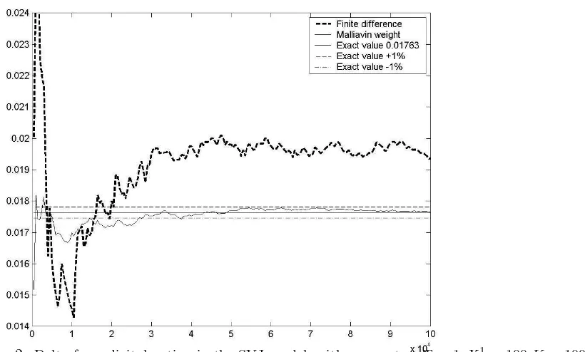
Stochastic volatility model with jump (SVJ) model
In Figures 2 we plot the delta for a digital option for an underlying that has a stochastic volatility with jumps (SVJ). The SVJ is an extension of the Heston model, where the stochastic volatility includes jumps. The sde are given by
dXt1 = rXt1−dt+qXt2−X
1
t−dWt1
X01 = x1
dXt2 = k(m−Xt2−)dt+σ q
X2
t−dW
2
t
+ Xt2− Z
R0
zµ˜(dz, dt)
X02 = x2.
The L´evy measure ofµ isν(z) =λe−a, thus the intensity of the Poisson processµis λand the
Figure 1: Delta for a digital option in the Bates model, with parametersT = 1, X1
0 = 100,K= 100,r= 0.05, σ= 0.04, X2
0 = 0.04, k= 1, m= 0.05, ρ=−0.8, λ= 1, a=−0.1 andb= 0.001
Figure 2: Delta for a digital option in the SVJ model, with parametersT = 1, X1
0 = 100,K = 100,r= 0.05, σ= 0.04, X2
It is obvious from the figures that the Malliavin weight performs better in the case of discontinues payoffs as we would expect.
A
Bounded derivative of the Picard approximation scheme
From inequality (20) we have
ξn+1(T)≤c1+
Z T
r
ξn(t)dt,
where c1 = cβ, c2 = cK2
T+ 1 +R
R0ρ
2(z)ν(dz) and ξ
n(t) = E[supr≤s≤t|DriXsn|2]. We will
prove by induction that
ξn(T)≤c1
n
X
j=0
cj2(T −r)j
j! . (26)
Forn= 0 it is obvious that (26) holds. Let (26) hold forn. Then
ξn+1 ≤ c1+c2
Z T
r
ξn(s)ds
≤ c1+c1c2
Z T
r n
X
j=0
cj2(s−r)j
j! ds
≤ c1+c1c2
n+1
X
j=1
cj2(T −r)j
j!
≤ c1
n+1
X
j=0
cj2(T−r)j
j!
Since limn→∞Pnj=0
cj2(T−r)j
j! =ec2(T−r)<∞, we can conclude that ξn(T)<∞.
B
Calculation of the Greeks for the SVJJ model
The system of stochastic differential equations of the extended Heston model can be rewritten in a matrix form:
dXt=b(t, Xt−)dt+σ(t, Xt−)dWt+
Z
R0
γ(t, z, Xt−)˜µ(dz, dt),
whereb∗(t, Xt−) = (rXt1−, k(m−Xt2−))∗,
σ(t, Xt−) =
Xt1−
q
Xt2− 0
σρqXt2− σp1−ρ2qX2
t−
and
Applying Lemma 8 we reach the result.
• DeltaThe first variation process has the following form
dYt = b′(t, Xt−)Yt−dt+σ
• Gamma In the case of the second derivative with respect the initial condition x by ap-plying again Lemma 9 to theDelta we reach our result.
• VegaIn order to calculateV ega we perturbXt withξ(t, x) =
. Furthermore, sinceXt2does not
depend onǫ we can deduce thatZt2 = 0. Thenβt=Yt−1Zt=
The Wiener directional derivative forqXs2− has the following form
D(0)t
Using Proposition 10 we reach the wanted expression.
• Alpha In order to calculate the sensitivity with respect to the jump amplitude we perturb Xt with ξ(t, x) =
. Following the same steps as inV ega we reach the wanted result.
References
[1] D Applebaum. L´evy Processes and Stochastic Calculus. Cambridge University Press, 2004. MR2072890
[3] K Bichteler, J Gravereaux, and J Jacod. Malliavin calculus for processes with jumps, vol-ume 2 of Stochastics Monographs. Gordon and Breach Science Publishers, New York, 1987. MR1008471
[4] M Davis and M Johansson. Malliavin Monte Carlo Greeks for jump diffusions. Stochastic Process. Appl., 116(1):101–129, 2006. MR2186841
[5] G Di Nunno, T Meyer-Brandis, B Øksendal, and F Proske. Malliavin calculus and antici-pative Itˆo formulae for L´evy processes. Infin. Dimens. Anal. Quantum Probab. Relat. Top., 8(2):235–258, 2005. MR2146315
[6] Y El-Khatib and N Privault. Computations of Greeks in a market with jumps via the Malliavin calculus. Finance Stoch., 8(2):161–179, 2004. MR2048826
[7] B Forster, E Luetkebohmert, and J Teichmann. Absolutely continuous laws of jump-diffusions in finite and infinite dimensions with applications to mathematical finance. arXiv, math.PR, 2005.
[8] E Fourni´e, J Lasry, J Lebuchoux, P Lions, and N Touzi. Applications of Malliavin calculus to Monte Carlo methods in finance. Finance Stoch., 3(4):391–412, 1999. MR1842285
[9] K Itˆo. Spectral type of the shift transformation of differential processes with stationary increments. Trans. Amer. Math. Soc., 81:253–263, 1956. MR0077017
[10] M Johansson. Malliavin Calculus for L´evy Processes with Applications to Finance. PhD thesis, Imperial College, 2004.
[11] J Le´on, J Sol´e, F Utzet, and J Vives. On L´evy processes, Malliavin calculus and market models with jumps. Finance Stoch., 6(2):197–225, 2002. MR1897959
[12] A Løkka. Martingale representation of functionals of L´evy processes.Stochastic Anal. Appl., 22(4):867–892, 2004. MR2062949
[13] D Nualart.The Malliavin calculus and related topics. Probability and its Applications (New York). Springer-Verlag, Berlin, second edition, 2006. MR2200233
[14] D Nualart and J Vives. Anticipative calculus for the Poisson process based on the Fock space. In S´eminaire de Probabilit´es, XXIV, 1988/89, volume 1426 of Lecture Notes in Math., pages 154–165. Springer, Berlin, 1990. MR1071538
[15] P Protter. Stochastic integration and differential equations, volume 21 of Stochastic Mod-elling and Applied Probability. Springer-Verlag, Berlin, 2005. Second edition. Version 2.1, Corrected third printing. MR2273672
[16] J Sol´e, F Utzet, and J Vives. Canonical L´evy process and Malliavin calculus. Stochastic Process. Appl., 117(2):165–187, 2007. MR2290191