www.elsevier.nlrlocatereconbase
The family as producer of health — an extended
grossman model
Lena Jacobson
)Departments of Community Medicine and Economics, Lund UniÕersity, Malmo¨rLund, Sweden
Received 7 May 1998; received in revised form 24 February 1999; accepted 30 November 1999
Abstract
Deriving a model, where each family member is the producer of his own and other family members’ health, shows that the family will not try to equalise marginal benefits and marginal costs of health capital for each family member. They will rather invest in health until the rate of marginal consumption benefits equals the rate of marginal net effective costs of health capital. The level of compensation in the social insurance system, the effective price of care, health related information, and transfer payments will all affect the production possibility set, and therefore the optimal level and distribution of family health.
q2000 Elsevier Science B.V. All rights reserved.
JEL classification: I1; I12
Keywords: Health; Human capital; Family; Grossman model
1. Introduction
Ž .
In his seminal work, Michael Grossman 1972a,b constructed and estimated a dynamic model of the demand for the commodity ‘good health’. He argued that
)Pfizer AB, PO Box 501, SE-183 25 Taby, Sweden. Tel.:¨ q46-8-519-064-05; fax:q 46-8-519-062-12.
Ž .
E-mail address: [email protected] L. Jacobson .
0167-6296r00r$ - see front matterq2000 Elsevier Science B.V. All rights reserved.
Ž .
such a model is important for two reasons. First, because the level of health influences the amount and productivity of labour supplied to an economy. Second, what consumers demand when they purchase medical services are not these services per se but rather ‘good health’. Added to these, there are further reasons. The model will help explain individuals’ health related behaviour, e.g., why some people smoke and some not, and why different individuals have different health
Ž .
and different health care utilisation Muurinen and Le Grand, 1985 . In order to evaluate and predict the effects of regulations, new technology, changes in social insurance schemes and government, and other programmes, knowledge about the effects on individuals’ demand for health and health related behaviour is essential. These effects will not be confined just to the present distribution of health capital Ždirect effects , but they will change the individual’s lifetime health profile. Žindirect effects . Hence, present and future total utilisation of health care re-. sources and social insurance are to a large extent the result of aggregate previous, present and future health related behaviour. Therefore, increasing our knowledge of what factors determine observed inequalities in health and the path of lifetime health has important policy implications.
Fundamental to the demand for health model is the sharp distinction between market goods and commodities. In this approach, consumers produce commodities
Ž .
with inputs of market goods and their own time Becker, 1965 . For example, they use sporting equipment and their own time to produce recreation, travelling time and transportation services to produce visits, and part of their Sundays and church services to produce ‘peace of mind’. Since goods and services are inputs into the production of commodities, the demand for these goods and services is a derived
Ž .
demand Grossman, 1972a, p. xv .
Further, the commodity good health is treated as a durable item, as one component of human capital. Health is demanded by the consumer for two reasons: as a consumption commodity, directly entering the individual’s utility
Ž .
function i.e., sick days being a source of disutility ; and as an investment commodity, determining the total amount of time available for market and nonmarket activities. According to the model, the level of health is endogenous,
Ž .
and depends at least in part on the resources allocated to its production. The shadow price of health will depend on many variables besides the price of medical care, and the quantity of health demanded will be negatively correlated with its shadow price.
Though the model yields valuable contributions to explain individuals’ health related behaviours and differences in health and health care utilisation, attempts to
Ž
develop the theoretical model have been relatively few for a review, see Gross-.
their health care utilisation.1 It also implies that the influence of other family members on the individual’s demand for health and demand for health care cannot be considered.
However, to analyse health issues from a family perspective is important for several reasons. It has been suggested that events during fetal life and early
Ž
childhood are associated with disease and mortality in later life Barker, 1992, .
1994; Power et al., 1996; Wadsworth, 1996, 1997 . The pathway linking early life with adult disease is explained by the process of ‘biological programming’ ŽBarker, 1992, 1994 and the continuities in lifetime socio-economic circum-. stances.2 This implies that a life course perspective is needed when searching for
the determinants of inequalities in health, and a demand for health model where the production of child health is included.
Further reasons for a family perspective, i.e., to include the influence other family members have on an individual’s health related behaviour, is supported by
Ž .
some empirical findings. Grossman 1975 found that an increase in wives’ schooling increased male health. Actually Grossman found the coefficient on
Ž
wives’ schooling to exceed the coefficient of men’s own schooling however, not
. Ž .
significantly higher . Currie and Gruber 1996 examined the effects of public health insurance on children’s health and utilisation of medical care. They found that parents with some college education are more likely to take their children to the doctor, with a stronger effect for mothers than for fathers, and that utilisation is higher both for first children and for children in smaller families. Further findings are that, conditional on household income, children in households with no male head have higher utilisation levels, and that visits seem to be normal goods while
Ž .
hospitalisations appear to be inferior goods. Thomas et al. 1991 found that a mother’s education has a large impact on child height in Northeast Brazil, and that almost all of this impact can be explained by indicators of her access to
Ž .
information. Delaney 1995 reports on negative effects of parental divorce on children’s health. Parental divorce also seems to have long-term effects on
Ž .
personality and longevity Tucker et al., 1997 .
Furthermore, how resources are allocated into investments in formal schooling and child health, as well as into investments in adult health and on-the-job
1
Ž .
Previously, for example Grossman 1975; see also Leibowitz, 1974 has argued that the health and intelligence of children partly depend on genetic inheritance, but that in particular they depend on early childhood environmental factors, which are shaped to a large extent by parents. However, Grossman et
Ž .
al. Becker, 1991; Cigno, 1991 view the increase in direct utility as the reason for parents’ investing in child quality, i.e., that child quality is a consumption commodity. This paper argues that there exists a monetary incentive as well.
2 Ž .
training, are decisions made jointly within the family. Existing demand for health models cannot explain and analyse such family and lifecycle related issues. Analysing health matters from a family perspective will be a step in the direction to a model in which the stocks of health and knowledge are simultaneously determined.3
This paper extends the Grossman model in that the family is seen as the producer of health4. By the family as producer of health is meant that each family
member is the producer, not only of his own health, but also of the health of other family members, and that not only his own income and wealth, but also the earnings of other family members, can be used in the production of health. The model will be derived assuming complete certainty. The implications of relaxing this assumption will be briefly discussed in the closing section of the paper.
According to Grossman, the individual receives both investment and consump-tion benefits from investing in his own health. This paper argues that this is valid also for investments in other family members’ health. Investment benefits occur
Ž .
because increased adult health or child health will decrease future time spent sick Žor time spent taking care of a sick child . Family time available for market work. will then increase, which may raise family income and increase consumption and investment possibilities for all family members. Consumption benefits may also occur, if family members derive utility not only from own health, but from the health of other members as well, i.e., the individual cares about the well-being of his or her child and spouse as he or she cares about his or her own well-being. Even though the individual may have incentives for producing health of other
Ž .
family members both with and without partly altruistic preferences , it is not self-evident how the objective function should be treated. While there is only one person who maximises his or her lifetime utility in the traditional Grossman individual demand for health model, there are at least two persons with common or non-common interests to consider, when formulating the optimisation problem in the family version of the model. In the model of the family as producer of
Ž
health developed in this paper, the family rather than the individuals making up .
the family is the economic unit, and a common preference approach will be used ŽBecker, 1974, 1991 . The implications of relaxing this assumption will be briefly. discussed in the final section of the paper.
Viewing the family as producer of health will not only affect how the benefits from investments in health are treated in the model, but also the household
3
ACurrently, we still lack comprehensive theoretical models in which the stocks of health and knowledge are determined simultaneously. I am somewhat disappointed that my 1982 plea for the
w Ž .x Ž .
development of these models has gone unanswered Grossman 1982 .B Grossman, 1998, p. 5 . 4
Ž .
production function s and the amount of available resources. In Grossman’s model, productivity is determined by the individual’s education. But seen from a family perspective, productivity may be determined by other family members’ education as well. Further, it may not be the individual’s education per se that determines his or her productivity in producing health, but human capital specific to that activity.5 Resources available for health production are not only own
income, but total family income. However, an important difference between investing in own health and investing in another person’s health is the difficulty to observe when ‘enough’ investments have been made; being uncertain whether enough has been done to restore the health of the other person. In contrast, for investments in own health, one knows when one prefers to use time and money to produce other commodities than health.6
To analyse an individual’s lifetime health and lifetime health care utilisation profile, it is necessary to use a lifecycle approach. A lifecycle approach may also be essential in order to explain observed differences in health and medical care utilisation among individuals. The lifecycle model concerns individual investment decisions and deals with resource allocation over an individual’s lifetime rather
Ž
than solely with decisions of the present time period see Polachek and Siebert Ž1993 for a description of the lifecycle human capital model, and how the.
.
lifecycle approach can be used to explain earnings variations . While an individ-ual’s amount of education and on-the-job training determine the individindivid-ual’s lifetime earnings, health capital determines not only the individual’s productivity but also his or her amount of healthy time. To tackle such a dynamic optimisation problem, there are three major approaches: calculus of variations, dynamic
pro-Ž .
gramming, and optimal control theory Chiang, 1992, pp. 17–22 . In this paper, optimal control theory will be used.
The paper is organised as follows. In Section 2, a model of the family as producer of health is derived in three steps. First, as a frame of reference, a model of the single person family is derived. Then, a model for the husband–wife family is derived and, eventually, a child is added to the family and a parents–child family model is presented. In Section 3, a graphic illustration of the family as producer of health model follows, and the effects on family health of changes in some exogenous variables are analysed. The paper concludes by a discussion of the implications of relaxing the assumption of common preferences and instead assumes allocation within the family to be the outcome of a cooperative Nash bargaining model, as well as a brief discussion of relaxing the assumption of complete certainty. Section 4 also includes some remarks regarding family
forma-5
For example self-management programs, educational programs for parents with chronically ill children, information about diet habits, etc.
6
tion, family size, and inter-sibling allocation, as well as a discussion of some policy implications.
2. The family as producer of health
In the following, a model of the family as producer of health will be developed successively in three steps. As a frame of reference, a model of the single person family will be presented, then the husband and wife family, and finally the parents and child family.7
In all three models, the family is assumed to choose the amount of market goods to consume in each time period in order to maximise family lifetime utility, given initial family wealth and each family member’s initial amount of health capital, and given the production functions and prices. The time path of family wealth and the paths of each family member’s health are then given by the optimal amounts of market goods chosen.
2.1. The single-person family
Ž .
Similar to Grossman 1972a,b , the individual is assumed to derive utility from own health, H , and from the consumption of other commodities8, Z . The
t t
individual has a strictly concave utility function, where utility in period t is
utsu H , Z .
Ž
t t.
Ž .
1The individual’s stock of health will depreciate during his or her lifetime, but
Ž .
the individual can invest in health produce health capital to offset this deprecia-tion in health capital. The individual’s stock of health will develop over time according to
EHtrEtsItydtH ,t
Ž .
27
The three versions of the family as producer of health model could be seen as tools for analysing health and health care utilisation during different stages in an individual’s life: as a child in a two
Ž
parents’ family; as a single adult person either prior to partnership, after a divorce, or at the end of
.
life ; as partners without children; and as partners with one child. The objective was not to analyse transitions between stages — that would have required quite a different analytical framework — and there are obviously many more possible stages to account for in real life. The objective was rather to make a model that could provide important insights into family health behaviour, given the fact that the family exists.
8
which is the equation of motion for the state variable health, and where dt is the rate of depreciation. The individual produces gross investments in health, I , andt
other commodities, Z , according to the production functions:t
Its
Ž
M , ht t , H; Et , H.
Ž .
3and
Zts
Ž
X , ht t , Z; Et , Z.
,Ž .
4where M and X are market goods9, and h and h are own time used in the
t t t, H t, Z
production of health and other commodities, respectively, Et, H and Et, Z are efficiency parameters10, and the production functions are assumed homogenous of
degree one in both goods and time inputs11.
Ž . Ž .
Individual family stock of wealth Wt will develop over time according to
EWtrEtsrWtqvt
Ž
H , Et t ,v.
ht ,vqBtyp Mt tyq X ,t tŽ .
5the equation of motion for the state variable wealth, where r is the market interest rate, vt is the wage rate, Et,v is the level of education and on the job training,
ht,v is time in market work, B is transfers, and p and q are the prices oft t t
Ž . Ž .
medical care Mt and other goods X , respectively.t
Health will affect market income in two ways: through its effect on the wage rate; and through its effect on healthy time available for market work. According
Ž .
to the formulation in Eq. 5 , an individual’s productivity in market work is determined by his or her amount of health capital and level of education and
Ž .
on-the-job training, implying that vt H , Et t,v can be thought of as the ‘labour market earnings rate of return on human capital’.
Ž . The available amount of healthy time in each time period is total time V less
Ž .
time spent sick ht, S , where time spent sick is determined by the individual’s
Ž Ž ..12 Ž .
amount of health capital ht, Ssht, S Ht . Time spent in market work ht,v , in
Ž . Ž . Ž .
producing health ht, H and other commodities ht, Z , and time spent sick ht, S
Ž . have to sum up to total time available V , i.e.,
Vsht ,vqht , Hqht , Zqht , S.
Ž .
69
Note that inputs in the production of health may not only be medical care services, but diet,
Ž .
exercise, housing, etc. See Grossman 1972a , for an analysis of joint production. Here, however, it will be assumed that medical care services are the only inputs in the production of health.
10
Ž .
In Grossman 1972a,b the individual’s productivity is determined by his or her level of schooling.
Ž . Ž
As in Becker 1991 , individual productivity in producing different commodities may differ activity
.
specific human capital . The individual’s productivity in producing health may depend on information and knowledge about health matters as well as the individual’s stock of health, while the individual’s
Ž
productivity in market work depends on his or her stock of educational capital formal education and
.
on-the-job training . 11
An assumption made by Grossman as well as his successors. 12
Eh rEH-0,E2h rEH2)0.
The individual’s problem is then to choose the time paths of the control variables M and Z that maximise lifetime utility. The problem can then bet t
written:
T yut
Max Us
H
e u H , ZŽ
t t.
tsuch that EHtrEtsIt , HydtHt
EWtrEtsrWtqvt
Ž
H , Et t ,v.
ht ,vqBtyp Mt tyq Xt tVsht ,vqht , Hqht , Zqht , S
H 0
Ž .
sH ,0 W 0Ž .
sW ,0 H and W given0 0H T
Ž .
sHTFHmin, W TŽ .
sWTG0, WTUlT ,Ws0T free
w
x
and X , Mt tG0 for all tg 0,T
Ž .
7where U is the individual’s intertemporal utility function, i.e., the discounted value of the individual’s lifetime utility, discounted by the individual’s rate of time preference, u. EHtrEt and EWtrEt are the equations of motion for the state
variables H and W, respectively, and V the time restriction. Hmin is the individual’s ‘death stock’ of health capital. The individual dies when health passes
Ž .
below some level Hmin, which determines T time of death . It should be observed that the individual is free to borrow and lend capital at each period, but the bequest ŽWT.cannot be negative.
Ž .
The solution to this horizontal-terminal-line problem Chiang, 1992 gives that the individual invests in health until the marginal benefit of new health equals the
Ž .
marginal cost of health see Appendix A :
eyutrl EurEHqh EvrEHy
Ž
wrl.
Eh rEHŽ
t ,W.
t t t ,v t t t t ,W t , S tsp dt tqry
Ž
EptrEt.
rpt ,Ž .
8Ž .
where lt,W and lt, H are costate variables, wt is the lagrange multiplier for the time restriction, EutrEH is marginal utility of health capitalt 13, EvtrEH is thet
marginal effect of health on wage14,Eht, SrEH is the marginal effect of health ont
the amount of sick time andpt is the effective price of medical care goods and Ž .
services M .t
Ž .
The first order condition A10 in the Appendix A gives that lt, H equals
Ž .
lt,Wpt. Thus, in periods when the budget is binding lt,W high or the effective
13
EurEH)0,E2urEH2-0.
t t t t
14
Ž .
price of care pt is high, lt, H will be high, implying that the individual’s stock of Ž .
health is low. Further, the first order condition A7 shows that:
Elt , HrEtslt , Hdtylt ,Wht ,v
Ž
EvtrEHt.
qwtŽ
Eht , SrEHt.
yŽ
EutrEH et.
yut,9
Ž .
i.e., the time path of lt, H will depend on, for example, the rate of depreciation in Ž .
health dt , the sensitivity in the individual’s wage rate to changed health
ŽEvtrEH , and the individual’s valuation of time how binding the time restrictiont. w
Ž .x
is wt . An increased rate of depreciation will increase lt, H, decreasing the individual’s level of health. If the individual’s wage rate becomes more sensitive
Ž .
to differences in health, the individual will invest more in health lt, H decreases . Finally, the more restricting the time constraint is, the higher will the individual’s
Ž .
valuation of time be wt , and the more will the individual invest in health Ždecreasing lt, H..
Note that whileEutrEH is the increase in utility in period t if health capital int
period t is increased by one unit, lt, H is the increase in lifetime utility if health in period t is increased by one unit of health capital.
Looking at the time path of the costate variable lt,W, the solution shows that
lt,W decreases over time with a rate equal to the rate of interest, r. According to the present formulation, the individual is free to borrow and lend capital at each
Ž .
[image:9.595.94.339.324.436.2]period of time EWtrEt can take both positive and negative values , but WT is
Fig. 1. An illustration of the paths of the control variable, c, and the state variable, y, in an optimal
Ž . Ž .
control problem. a Illustrates that the control path, c t , does not have to be continuous; it only has to be piecewise continuous. For example, an individual’s medical care consumption can make jumps over
Ž .
time, i.e., be positive in some time periods and zero in some. The state path, y t , on the other hand,
w x Ž .
has to be continuous throughout the time period 0,T as illustrated in b . However, the state path is allowed to have a finite number of sharp points, i.e., it needs to be piecewise differentiable. Those sharp points will occur at the times when the control path makes a jump. For example, a jump in
Ž .
medical care consumption, say at time t , may correspond to a sharp decrease in health, y t . To place1 1 a state-space constraint on the maximisation problem can, for example, be to only allow for positive
Ž . Ž
values on y t , i.e., the permissible area of movement for y is the area above the horizontal axis for
. Ž
example, if y is monetary wealth, to allow for saving but not for borrowing . Source: Chiang 1992, p.
.
restricted to be non-negative, i.e., the bequest cannot be negative. If formulating
Ž .
the problem as a state-space constraint problem Chiang, 1992, pp. 298–300 ,
EWtrEt is forced to be non-negative in every period. lt,W will then not be
Ž
continuous, but make jumps in periods where this restriction is binding see Fig. 1 .
for an illustration .
The values of lt,W and wt may be interpreted as measures of stress, economic and time stress, respectively. If the wealth andror time constraint is binding for several periods, the values of lt,W and wt will be high and increasing.
2.2. The husband–wife family
Using a common preference model of family behaviour, the instantaneous
Ž .
family strictly concave utility function can be written as
usu H , H , Z ,
Ž
m f.
Ž
10.
where time subscripts are omitted in order to simplify the notations. u is family
Ž . Ž .
utility in period t, Hm and H are husband male and wife female health,f
respectively, and Z is a vector of commodities consumed. As in the single-person
Ž . Ž .
model, the depreciation in male dm and female health df may be offset by
Ž . Ž .
gross investments in male Im and female If health, respectively, according to the production functions:
ImsIm
Ž
M , hm H m ,m, hH m ,f; EH ,m, EH ,f.
Ž
11.
and
IfsIf
Ž
M , hf H f ,m, hH f ,f; EH ,m, EH ,f.
,Ž
12.
where the production functions are assumed homogenous of degree one in goods and time inputs. Mmand M indicate market goods used in the production of malef and female health, respectively. Time used in the production of health is indicated by hH m,m, hH m,f, hH f,m, and hH f,f. The first subscript denotes what is produced;
Ž . Ž .
male Hm or female Hf health, the second subscript denotes who is the
Ž . Ž .
producer; the husband m or the wife f . EH ,m and EH ,f indicate male and female productivity in health production. Similarly, net investments in health are
EHmrEtsImydmHm
Ž
13.
and
EHfrEtsIfydfH .f
Ž
14.
The development of family wealth follows
EWrEtsrWqvm
Ž
H , Em v,m.
hv,mqvfŽ
H , Ef v,f.
hv,fqBŽ . Ž . Ž wherevm H , Em v,m and vf H , Ef v,f are the husband’s and wife’s wage rates or
. Ž .
labour market earnings rates of return on human capital , respectively. Ev,m Ev,f
Ž . Ž .
is the husband’s wife’s level of education and on-the-job training, and hv,m hv,f
Ž .
his her amount of time spent in market work. The time restrictions are
Vishv,iqhZ ,iqhH m ,iqhH f ,iqhS ,i ism,f.
Ž
16.
Ž .
Total time for each spouse Vi is allocated between time spent in market work Žhv,i., in home production of health hŽ H m,iqhH f,i. and other commodities hŽ Z,i.
Ž .
and time being sick hS,i , where health determines the amount of sick time ŽhS,ishS,iŽHi...
The problem facing the family is to choose the time paths of the control variables M , M , and Z, in order to maximise lifetime utility. The problem canm f
Ž .
then be written time subscripts still omitted for simplicity :
T yut
Max Us
H
e u H , H , ZŽ
m f.
tsuch that EHmrEtsImydmHm
EHfrEtsIfydfHf
EWrEtsrWqvm
Ž
H , Em v,m.
hv,mqvfŽ
H , Ef v,f.
hv,fqByp M
Ž
mqMf.
yqXVishv,iqhZ ,iqhH m ,iqhH f ,iqhS ,i ism,f
Hm
Ž .
0 , H 0 , W 0 givenfŽ .
Ž .
Hm
Ž .
T andror H TfŽ .
FHminW T G0, WUlW
s0
Ž .
T TT free
w
x
and X , M , Mm fG0 for all tg 0,T
Ž
17.
.T , in this case, is the ‘lifetime’ of the husband–wife family; the family ‘dies’ when husband andror wife no longer has a health status greater than Hmin. The
Ž
solution to this maximisation problem gives the marginal condition see Appendix .
A, condition A16 :
w x
Ž . Ž . Ž . Ž .
EurEHm pmŽdmqry EpmrEt rpm.y EvmrEHm hv,my wmrlW EhS ,mrEHm
s .
w x
Ž . Ž . Ž . Ž .
EurEHf pfŽdfqry EpfrEt rpf.y EvfrEH hf v,fy wfrlW EhS ,frEHf
18
Ž
.
Ž .
Thus, the optimal condition 8 , i.e., that the individual invests in health until marginal benefits equal marginal costs, is not valid any more. In a two-person family with common preferences, husband and wife together invest in health until
Ž Ž ..
Ž .
rate of marginal net effective cost of health capital right hand side . The net effective cost of health capital equals the user cost of capital less the marginal
Ž . Ž Ž .
investment benefit of health capital in brackets . A similar result see Eq. A10 .
in Appendix A can be derived for lifetime utility of health, i.e., that
lWslH mrpmslH frpf.
Ž
19.
Ž .
Condition 19 implies that family members will invest in health until the rate of
Ž .
marginal lifetime utility of health to the effective price of health is equal for all
Ž .
family members and equal to the marginal utility of wealth .
2.3. The parents–child family
Adding a child to the husband–wife family model gives the following
instanta-Ž .
neous strictly concave family utility function time subscripts omitted :
usu H , H , H , Z ,
Ž
m f c.
Ž
20.
where Hc is child health, developing over time according to the equation of motion,
EHcrEtsIcydcH ,c
Ž
21.
Ž .
and produced by the child’s parents by use of market goods Mc and parental
Ž .
time hH c,m and hH c,f, respectively according to the production function:
IcsIc
Ž
M , hc H c ,m, hH c ,f; EH ,m, EH ,f.
.Ž
22.
Ž .
The time restriction for each parent husband and wife, respectively then becomes
Vishv,iqhZ ,iqhH m ,iqhH f ,iqhH c ,iqhS ,iqhSc ,i ism,f
Ž
23.
where hSc,iis time taking care of a sick child for parent i, and whereEhSc,irEHc-0 and E2h rEH2)0.15 The family problem will now be extended to choose the
Sc,i c
paths of M , M , M , and Z in order tom f c
T yut
Max Us
H
e u H , H , H , ZŽ
m f c.
tsuch that EHjrEtsIjydjHj for jsm, f, c
EWrEtsrWqvm
Ž
H , Em v,m.
hv,mqvfŽ
H , Ef v,f.
hv,fqByp M
Ž
mqMfqMc.
yqXVishv,iqhZ ,iqhH m ,iqhH f ,iqhH c ,iqhS ,iqhSc ,i for ism,f
H 0j
Ž .
given for jsm,f,c15
H Tj
Ž .
FHmin for at least one of jsm,f,cU
W T
Ž .
G0, W TŽ .
lWŽ .
T s0T free
w
x
and X , MjG0 for all tg 0,T , jsm,f,c.
Ž
24.
As in the previous case, T is the ‘lifetime’ of the parents–child family.16
Ž . Ž
Solving the maximisation problem in Eq. 24 adds the marginal condition see .
Appendix A, condition A18 ,
EurEHi EurEHc
w x
p diŽ iqryŽEpirEt.rpi.y ŽEvirEH hi. v,iyŽwirlW. ŽEhS ,irEHi.
s ism ,f
w x
p dcŽ cqryŽEpcrEt.rpc.y yŽwmrlW. ŽEhSc ,mrEHc.yŽwfrlW. ŽEhSc ,frEHc.
25
Ž
.
Ž .
to the one in Eq. 18 . The net effective marginal cost of adult health capital is the Ž .
same as in condition 18 . Net effective marginal cost of child health is equal to the user cost of child health capital less the marginal investment benefit of child health, which is the sum of the monetary value of the change in time taking care of a sick child for father and mother, respectively, for a marginal change in child
Ž .
health. Condition 19 is now extended to
lWslH mrpmslH frpfslH crpc,
Ž
26.
implying that the family invests in health until the rate of marginal utilities of Žlifetime health to effective price of health for all family members is equal and. equal to the marginal utility of wealth. The family will not try to equalise the amount of health capital between family members.
Ž .
Rearranging condition 26 gives that lH csl pW c, implying that poor families Žwhere the wealth restriction is binding value a marginal change in child health. higher than rich families, and that families for who the wealth constraint is not
Ž .
binding lWs0 has a zero marginal utility of child health. Further, it implies that a child with unhealthy parents can be expected to have lower health compared with a child with healthy parents, because resources have to be spent on increasing
Ž . the health of the unhealthy parents to achieve condition 25 .
16
Even though not directly included in the models above, for simplicity, an individual’s lifetime may be seen as consisting of three time periods. In the first time period, the individual is a child in a parents–child family; in the second period, he or she is a parent in the parents–child family; and in the
Ž .
third period, he or she is a husband or wife in the husband–wife family. His her initial health in the
Ž . Ž .
first period is his her inherited amount of health capital. Initial health in the second period is his her
Ž . Ž
terminal amount of health in the first period and so on. This imply that his her health as old in the
. Ž . Ž .
third period is determined by inherited health, investments made by his her parents during his her
Ž . Ž .
3. Graphic illustrations of the model
3.1. The optimal distribution of family health
Ž .
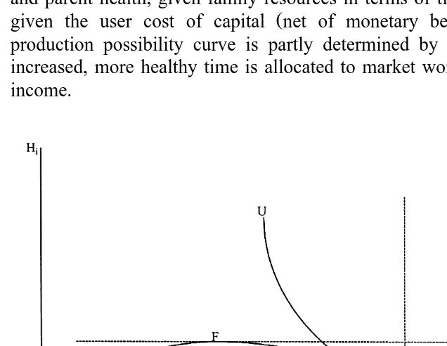
The maximisation problem in Eq. 24 is illustrated in Fig. 2, assuming a family consisting of one parent and one child, and for a given amount of Z. Parent health ŽHi.is measured on the vertical axis and child health HŽ c.on the horizontal axis.
Ž .
The slope of the production possibility curve AB is given by the right hand side Ž .
of Eq. 25 , i.e., the ratio of marginal net effective cost of adult health and marginal net effective cost of child health. UU is an indifference curve represent-ing the level of family utility, with the slope given by the left hand side of Eq. Ž25 ..
The production possibility curve AB gives all possible combinations of child and parent health, given family resources in terms of time and initial wealth, and
Ž .
[image:14.595.58.376.268.514.2]given the user cost of capital net of monetary benefit . The shape of the production possibility curve is partly determined by the fact that as health is increased, more healthy time is allocated to market work, which increases family income.
Fig. 2. An illustration of the solution to the maximisation problem in Section 2 given by the marginal
Ž .
condition in Eq. 25 . This illustration assumes a family consisting of one parent and one child, and is
Ž . Ž .
If all time and wealth were allocated to the production of child health, the distribution of health would be given by point B. Producing one amount of parent health using some of total family time and wealth would reduce adult sick time and increase family income, allowing child health to increase as well. It would be
Ž
possible to increase both child and adult health at the same time given time, .
wealth and user cost of capital until health states defined by point D were reached. Then, increased adult health would be so ‘expensive’ that child health had to be reduced to make additional investments in adult health possible. If child health was reduced enough to allow for the production of adult health given by point F, the parent would have to spend so much time taking care of the sick child that income would no longer be enough to make gross investments compensating for the depreciation, and child and adult health would both fall.
For completely selfish parents, child health per se would not enter the family Ž utility function, so indifference curves would be horizontal. Maximising utility for
. Ž .
given Zt subject to the production possibility set budget constraint would then give point F in Fig. 2. This shows that even a selfish parent would invest in child
Ž
health, but only because child health affects family income the investment aspect .
of child health . However, because of altruism, adult utility will increase as child health increases. For a completely altruistic parent, indifference curves would be vertical. Maximising family utility then implies that the parent would be willing to invest in child health until point D is reached. Thus, altruism would be effective along the production possibility curve from F to D. The location of point P on the production possibility curve between F and D will depend on the parent’s degree of altruism toward the child; ceteris paribus, a more altruistic parent would choose a point closer to D than a less altruistic parent.
If point E represents the endowed amounts of health capital at the beginning of period t, the adult would invest in both own and child health until point P was reached. However, assume that adult health cannot be increased because of, for example, lack of treatment. Then the adult would maximise utility by investing in child health until point O is reached.
If, at the beginning of time t, their endowed amounts of health capital were as represented by point O, then the parent would invest in own health only and let child health depreciate until point P was reached. It may then look as if the parent underinvested in child health, but this would be a utility maximising behaviour given the restrictions he or she were faced with.
Because the health of one of the individuals could be increased without
Ž .
decreasing the health of the other, points on the segments AF and BD in Fig. 2 do not represent stable situations. Health given by points on these positive sloping parts of the production possibility curve would only be stable if additional gross investments in health, to offset depreciation, could not be made because of, for example, lack of treatment. In this paper, it is assumed that the individuals always have this possibility, i.e., the analyses focus on the negatively sloping part of the
Ž .
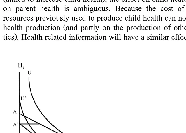
3.2. Effects of changes in exogenousÕariables on optimal family health
Ž
An increased rate of depreciation, d or an increased coinsurance rate in the .
health insurance system, increased p that increasesp would affect family health by increasing the net cost of health capital. If both child and parent depreciation rates increased, but dc increased more than dm, the point indicating optimal health would move from P to PX in Fig. 3. The income effect would decrease both child and parent health, but the substitution effect would increase parent health while decreasing child health. The total effect would be a reduction in child health, while the effect on parent health would be ambiguous. Using Fig. 3 to analyse the effect of a reduction in the coinsurance rate for medical care utilisation by children Žaimed to increase child health , the effect on child health is positive but the effect. on parent health is ambiguous. Because the cost of child health is reduced, resources previously used to produce child health can now partly be spent on adult
Ž
health production and partly on the production of other consumption commodi-.
ties . Health related information will have a similar effect. Increased health related
[image:16.595.60.379.260.489.2]Ž .
Fig. 3. This figure illustrates the effects of changes in the costs of health capital. Parent health Hi is
Ž .
given by the vertical axis and child health Hc by the horizontal axis. The initial production possibility curve is given by AB; UU and UXUXare family indifference curves; and initial optimal health is given by point P. An increased cost of health, where the cost of child health increases more than the cost of parent health, will give the new production possibility curve AXBX, and a new equilibrium given by
X
Ž
point P . The total effect on family health can be divided into an income effect the move from P to Y
. Ž Y X
information will make the parent more productive in producing new health. This increase in EH ,i will decrease bothpi andpc.
Ž
If the value of parent time is set equal to his or her wage rate i.e,.wirlWsvi, .
ism,f and if some insurance exists, covering x% of losses due to taking care of a sick child, the net cost of child health will be:
p dc
Ž
cqryŽ
EpcrEt.
rpc.
y yvm
Ž
EhSc ,mrEHc. Ž
1yx.
yvfŽ
EhSc ,frEHc. Ž
1yx.
.Ž
27.
Ž .
For x)0, the net cost of child health in Eq. 27 is higher than the net cost of
Ž . Ž .
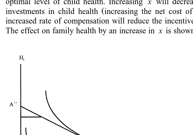
child health in Eq. 25 the denominator on the right hand side , implying a lower optimal level of child health. Increasing x will decrease the monetary value of
Ž .
[image:17.595.56.379.241.468.2]investments in child health increasing the net cost of child health because an increased rate of compensation will reduce the incentive to invest in child health. The effect on family health by an increase in x is shown in Fig. 4. Optimal health
Fig. 4. This figure illustrates the effects of an increase in the rate of compensation for income losses
Ž . Ž .
due to taking care of a sick child x and an increase in transfer payment B , respectively. The
increase in the level of compensation will increase the slope of the production possibility curve from X
Ž . X
AB to AB , increasing the net cost of child health H . Optimal health will move from point P to P .c
Ž .
will move from P to PX. The effect on child health is negative while the effect on parent health is ambiguous. The reason for this reduction in child health is that the parent cannot increase family income as much as before by investing in child health after x is increased. An increase in the compensation for losses due to own Žparent illness will have a similar effect, but the reduction in H due to the. i increase in the level of compensation will now partly be offset by the reduction in the wage rate caused by the parent’s reduced health.
Ž .
An increase in transfer payment B has no effect on the marginal condition in Ž .
Eq. 25 , but it will have an effect on family health. As shown in Fig. 4, an increase in B will shift the production possibility curve to the right. As shown, an increase in B will increase both parent and child health, i.e., the point of optimal health will move from P to PY. As Fig. 4 is drawn, the increase in B is assumed to have no effect on the slope of the production possibility curve. However, it may be the case that an increase in B affects the parent’s time allocation decision, for example decreasing the incentive for market work. Such a decrease in hv,i will then lead to a flatter production possibility curve.
4. Discussion and concluding remarks
This paper has extended the individualistic demand for health model, the Grossman model, by deriving a model of the family as producer of health. This is an important extension because it makes it possible to analyse the influence that other family members may have on an individual’s health related behaviour and to analyse differences in health and health care utilisation between children.
This section summarises the conclusions and discusses the implications of some of the assumptions and simplifications made in the paper. It ends with a discussion of some policy implications of the model.
4.1. Conclusion
The purpose of this paper was to develop a demand for health model that takes into account characteristics and behaviour of other family members’ on an individual’s health and health care utilisation. This was done by treating each family member as a producer of his own and other family members’ health.
The extended model, the family-as-producer-of-health model, has several impli-cations. The main finding is that the family will not try to equalise marginal benefits and marginal costs of health capital for each family member. Instead, they will invest in health until the rate of marginal consumption benefits equals the rate of marginal net effective costs of health capital, or, in other words, family
Ž .
Ž
to the effective price of health is equal for all family members and equal to the .
marginal utility of wealth . The net effective cost of health capital equals the user cost of capital less the marginal investment benefit of health capital. Variables such as the level of compensation in the social insurance system, the effective price of care, health related information, and transfer payments will all affect the family production possibility set, and, therefore, the optimal level and distribution of family health.
Ž .
Results related to individual health show a that an increased rate of deprecia-Ž .
tion will decrease the individual’s level of health; b that when an individual’s wage rate becomes more sensitive to differences in health, the individual will
Ž .
invest more in health; and c that the more restricting the time constraint is, the higher the individual’s valuation of time will be and the more the individual invest in health.
Ž
Regarding child health, it is shown that poor families where the wealth .
restriction is binding value child health higher than rich families and that families where the wealth constraint is not binding have a zero marginal utility of child health. Further, a child with unhealthy parents can be expected to have lower health compared with a child with healthy parents, because resources have to be spent on increasing the health of the unhealthy parents for the marginal condition to be fullfilled. It is also shown that even a selfish parent will invest in child health
Ž .
because child health affects family income the investment aspect of child health . By assuming that adult health cannot be increased because, for example, lack of treatment, it is shown that the adult will maximise utility by ‘overinvesting’ in child health. If, on the other hand, their endowed amounts of health capital were such that the child’s health was above and the parent’s health below what is regarded as optimal, the parent will invest only in own health and let child health depreciate until optimum is reached.
The effects of changes in some exogenous variables on optimal family health were also considered in the paper. An increased rate of depreciation, an increased coinsurance rate in the health insurance system, or an increase in health related information will affect family health by increasing the net cost of health capital.
4.2. Common preferences
The model derived in this paper is based on the assumption of common
Ž .
preferences Becker, 1991 . As shown by recent empirical work, it may not be a proper description to assume that spouses have common preferences and to assume that who has the control of resources has no impact on how these resources are allocated. Empirical work shows, for example, that the distribution
Ž .
of non-earned income does matter. Thomas 1990 found that unearned income in the hands of a mother had a bigger effect on her family’s health than income under
Ž .
parental education and child height. He found that the education of the mother had a bigger effect on her daughters’ height, while paternal education had a bigger impact on his sons’ height. He also found that as the woman’s power in the household allocation process increased17, she became more able to assert her preferences and direct more resources towards commodities she cares about.
Ž .
Haddad and Hoddinott 1994 used a non-cooperative bargaining model to exam-ine the impact of the intrahousehold distribution of income on the anthropometric
Ž .
status height-for-age of boys relative to girls. They found that an increase in female share of household income seemed not to be gender neutral; boys would gain relative to girls.
Ž Several models of family behaviour have been suggested in the literature for
.
surveys, see Lundberg and Pollak, 1996 and Bergstrom, 1997 . McElroy and
Ž .
Horney 1981; see also Manser and Brown, 1980 suggested a model where the distribution of resources within the family is seen as the outcome of a cooperative Nash bargaining process. According to this bargaining model, the objective of the spouses is to maximise a utility–gain production function, defined as the product of the husband’s gain and the wife’s gain from marriage. These gains from
Ž .
marriage will decrease when utility as single the threat point increases.
Then, using a Nash bargaining model to describe family behaviour, the effect on family health of an increase in the non-earned income by the wife is illustrated
Ž . Ž .
in Fig. 5. Male health Hm is given by the horizontal axis, and female health Hf
by the vertical axis. An increase in the non-earned income by the wife will shift the production possibility curve outwards as in the common preference case in Fig. 4. However, in this case, an increase in non-earned income will also affect the
Ž .
iso–gain product curve the bargaining analogue of indifference curves through its effect on the threat-point. If utility as single is the actual threat-point, her bargaining power will increase, because the increase in her non-earned income will increase her utility as single. The iso–gain product curve will twist from NN to NYNY. Compared to the common preference model, the increase in female health will be larger, HfYyH compared to Hf fXyH . The increase in the mother’sf
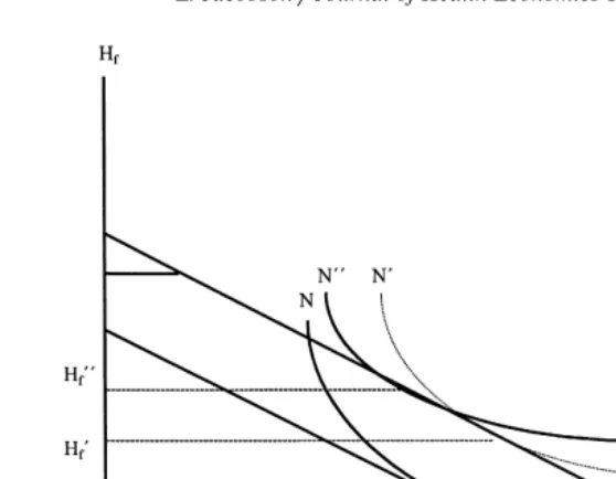
non-earned income may also increase child health either because she cares more about child health than the father does, or because she prefers more healthy goods than he does. In the last case, not only child health will increase, but the health of all family members. Thus, according to the Nash bargaining model, family decisions are the outcome of some bargaining process and family demands will depend not only on prices and total family income, but also on the determinants of the threat points18.
17
As indicators of power in the household allocation decisions the study used nonlabour income, opportunities outside the home, and relative educational status.
18 Ž .
Fig. 5. An illustration of how distribution is determined according to the Nash bargaining model. Male
Ž . Ž .
health Hm is given by the horizontal axis, and female health Hf on the vertical axis. An increase in the non-earned income by the woman will shift the production possibility curve out as in the common
Ž .
preference case in Fig. 4 the increase in transfer payment . However, in this case, an increase in
Ž
non-earned income will also affect the iso–gain product curve the bargaining analogue of indifference
. Y Y
curves through its effect on the threat-point. The iso–gain product curve will twist from NN to N N . Compared to the common preference model, the increase in female health will be larger, HfYyHf compared to HfXyH . If her threat-point is unaffected by this increase in non-earned income, the newf iso-gain product curve is given by the dashed curve NXNX.
4.3. Other assumptions and simplifications
In order to focus on the implications of extending the individual demand-for-health model to a family model, the model was derived assuming complete
Ž .
certainty. An individual or a family may face three types of uncertainty in health. Ž
First, there is uncertainty as to the current size of the health capital a characteris-. tic which the individual shares with his or her professional health care agents . Second, there is uncertainty about the rate of depreciation of the health capital. Third, there is uncertainty about the effects of the various inputs in the health production function on the health capital. The first type of uncertainty does not seem to have been introduced in any formal models. The second andror the third types have been included in various ways in formal models developed by Cropper Ž1977 , Dardanoni and Wagstaff 1990 , Selden 1993 , Chang 1996 , Liljas. Ž . Ž . Ž . Ž1998 , and Picone et al. 1998 . In an uncertain world, risk-averse individuals. Ž .
Ž .
they would in a perfectly certain world. This result is quite in accordance with the
Ž .
discussion in Grossman 1972a,b , even though it was not formally proved, since the original Grossman model ruled out uncertainty for the sake of simplicity.19A
Ž .
portfolio approach to health behaviour has been discussed by Dowie 1975 and,
Ž .
more formally, by Horgby 1997 . Their basic message is that the individual should diversify his or her health investment activities, if there is uncertainty about the effects on health capital of various measures intended to improve health.
Some implications of these results for the model developed in this paper seem
Ž .
to be worth noticing. The expected total health capital of the family would be larger than in the certain case. With common preferences, the relative distribution
Ž .
of expected health capital among family members would remain the same as in the certain case. With non-common preferences, however, the relative distribution may change, since family members may then have different attitudes towards risk and uncertainty. For the same reason, the optimal portfolio of health investments may be quite different for different family members, not only because of the characteristics included in the certain case developed in this paper but also depending on diverging attitudes towards risk among family members. Thus, this phenomenon may contribute to explaining differing morbidity and mortality expectations and experiences among family members.
A further simplification made in the paper is that important family related
Ž .
decisions such as family formation i.e., marriage or divorce , family size and inter sibling allocation of resources were not considered. Those issus are discussed by
Ž . Ž . Ž .
Becker 1991 , Becker and Lewis 1973 and Becker and Tomes 1976 , and give Ž
rise to issues such as assortative marriage that equally healthy or wealthy .
individuals marry each other , the interaction between quantity and quality of children, and whether the transfers of resources from parents to children are based on efficiency or equity considerations.
4.4. Policy implications
The model presented in this paper has some important policy implications when discussing and analysing differences in health and health care utilisation among individuals and for a single individual over time. It was shown that variables such as other family members’ health, preferences, education, income, etc., are
impor-Ž
tant for an individual’s stock of health and health care utilisation i.e., health .
related behaviour . It was further shown that an individual’s present health and health care utilisation is the result of investments made earlier in life by him or herself, and by his or her parents.
19
Grossman suggested that the simplest way to introduce uncertainty might be to let a given
Ž .
Consequently, the individual’s family situation has to be considered when formulating prevention, treatment, rehabilitation and educational health pro-grammes. But family variables also have to be included in the evaluation of such programmes and in analyses of reasons to differences in health and health care utilisation.
Naturally, the extended theoretical model also calls for new empirical estima-tions, which can increase our knowledge about health behaviour both per se and in policy-relevant contexts. Some preliminary results are available in Bolin et al. Ž1998a , who analyse the demand for health and health care in Sweden 1980. r81 and 1988r89, using a Swedish panel data set and considering both the dynamic character of the Grossman model and the impact of the family structure.
Acknowledgements
I am grateful for the helpful comments and suggestions on earlier drafts from Bjorn Lindgren, Kristian Bolin, Inga Persson, participants at the seminar in
¨
political economy at the Department of Economics, Lund University, and two referees. This research was supported by grants from Vardalstiftelsen and from the Swedish National Institute of Public Health, which is gratefully acknowledged.Appendix A
To solve the dynamic optimisation problem in Section 2, optimal control theory
Ž .
is used Chiang, 1992 . The problem is formulated as an equality constraint problem where time is binding in each period, but where the family is free to borrow and lend during the family lifetime. It contains given initial points, but a variable terminal point; i.e., a horizontal-terminal line problem. The Lagrangian
Ž .
for solving this problem is Chiang, 1992, p. 276 :
Lsu H , H , H , Z e
Ž
m f c.
yutqlH m Im
Ž
M , hm H m ,m, hH m ,f; EH ,m, Eh ,f.
ydmHmqlH f If
Ž
M , hf H f ,m, hH f ,f; EH ,m, EH ,f.
ydfHfqlH c Ic
Ž
M , hc H c ,m, HH c ,f; EH ,m, EH ,f.
ydcHcqlW rWqvm
Ž
H , Em v,m.
hv,mqvf
Ž
H ,Ef v,f.
hv,fyp MŽ
mqMfqMc.
yqXw
x
qwm Vyhv,myhZ ,myhH m ,myhH f ,myhH c ,myhS ,myhSc ,m
w
x
Ž . F.O.C interior solution
w
x
ELrEMsELrEXs0 for all tg 0,T
ELrEwmsELrEwfs0
EHmrEtsELrElH m equation of motion for the state variable Hm
EHfrEtsELrElH f equation of motion for the state variable Hf
EHcrEtsELrElH c equation of motion for the state variable Hc
A2
Ž
.
EWrEtsELrElW equation of motion for the state variable WElH mrEts yELrEHm equation of motion forlH m
ElH frEts yELrEHf equation of motion forlH f
ElH crEts yELrEHc equation of motion forlH c
ElWrEts yELrEW equation of motion forlW
These F.O.C.’s then give:
ELrEMjslH jEIjrEMjylWps0 jsm,f,c
Ž
A3.
ELrEXseyutEurEZEZrEXylWqs0
Ž
A4.
ELrElH jsI M , hj
Ž
j H j,m, hH j,f; EH ,m, EH ,f.
ydjHj jsm,f,cŽ
A5.
ELrElWsrWqvm
Ž
H , Em v,m.
hv,mqvfŽ
H , Ef v,f.
hv,fyp M
Ž
mqMfqMc.
yqXŽ
A6.
ELrEHsEurEH eyutyl dql h EvrEHywEh rEH
i i H i i W v,i i i i S ,i i
s yElH irEt ism,f
Ž
A7.
ELrEH sEurEH eyut
yl d yw Eh rEH yw Eh rEH
c c H c c m Sc ,m c f Sc ,f c
s yElH crEt
Ž
A8.
ELrEWslWrs yElWrEt
Ž
A9.
Ž . Rewriting Eq. A3 gives:
lH jslWpr
Ž
EIjrEMj.
sl pW j jsm,f,cŽ
A10.
Ž .
and the time derivative of Eq. A10 :
ElH jrEtsElWrEtpjqlWEpjrEt jsm,f,c
Ž
A11.
Ž .
Solution to the single person family problem: setting Eq. A7 equal to Eq. ŽA11 , for j. si, gives
EurEH eyutyl dql h E rEH yw Eh rEH
Ž
i.
H i i W v,iŽ
v,i i.
iŽ
S ,i i.
Ž . Ž .
and using Eqs. A10 and A9 to substitute for lH m and yElWrEt gives
Žsubscript i omitted.
EurEH eyutyl pdql h EvrEH yw Eh rEH
Ž
.
W W vŽ
.
Ž
S.
slWrpylW
Ž
EprEt.
Ž
A13.
Ž .
Re-arranging Eq. A13 and adding the time subscript gives the marginal condition Ž .
in Eq. 8 , i.e.,
eyut
rl EurEHqh EvrEHy
Ž
wrl.
Eh rEHŽ
t ,W.
t t t ,v t t t t ,W t , S tsp dt tqry
Ž
EptrEt.
rpt .Ž
A14.
Ž . Ž .
Solution to the husband–wife family problem: use Eqs. A9 – 11 to write Eq. ŽA7 as.
EurEH eyutyl p d ql h EvrEH yw Eh rEH
Ž
i.
W i i W v,iŽ
i i.
iŽ
S ,i i.
slWrpiylW
Ž
EpirEt ,.
ism,f.Ž
A15.
Set i equal to m and f, respectively, and divide the expression for m with the one Ž .
for f to obtain the marginal condition in Eq. 18 ,
w x
Ž . Ž . Ž . Ž .
EurEHm pmŽdmqry EpmrEt rpm.y EvmrEHm hv,my wmrlW EhS ,mrEHm
s .
w x
Ž . Ž . Ž . Ž .
EurEHf pfŽdfqry EpfrEt rpf.y EvfrEH hf v,fy wfrlW EhS ,frEHf
A16
Ž
.
Ž . Ž .
Solution to the parents–child family problem: use Eqs. A9 – 11 to write Eq. ŽA8 as:.
EurEH eyutyl p d yw Eh rEH yw Eh rEH
Ž
c.
W c c mŽ
Sc ,m c.
fŽ
Sc ,f c.
slWrpcylW
Ž
EpcrEt.
Ž
A17.
Ž . Ž .
The marginal condition in Eq. 25 is then obtained by dividing Eq. A15 for
Ž .
ism with Eq. A17 , i.e.,
EurEHm
EurEHc
w x
Ž . Ž . Ž . Ž .
pmŽdmqryEpmrEt rpm.y EvmrEHm hv,my wmrlW EhS ,mrEHm
s .
w x
Ž . Ž . Ž . Ž . Ž .
p dcŽ cqryEpcrEt rpc.y y wmrlW EhSc ,mrEHc y wfrlW EhSc ,frEHc
A18
Ž
.
References
Ž .
Barker, D.J.P. Ed. , 1992. Fetal and infant origins of adult disease. British Medical Journal, London. Barker, D.J.P., 1994. Mothers, babies, and disease in later life. British Medical Journal, London. Becker, G.S., 1965. A theory of the allocation of time. The Economic Journal 75, 493–517.
Ž .
Becker, G.S., 1991. A Treatise on the Family. Harvard University Press, Cambridge, MA, enlarged edition.
Becker, G.S., Lewis, H.G., 1973. On the interaction between the quantity and quality of children.
Ž .
Journal of Political Economy 81 2 , 279–288, Pt. 2.
Becker, G.S., Tomes, N., 1976. Child endowments and the quantity and quality of children. Journal of
Ž .
Political Economy 84 4 , S143–S162, Pt. 2.
Ž .
Bergstrom, T., 1997. A survey of theories of the family. In: Rosenzweig, M.R., Stark, O. Eds. , Handbook of Population and Family Economics. North-Holland, Amsterdam.
Bolin, K., Jacobson, L., Lindgren, B., 1999. The demand for health and health care in Sweden 1980r81 and 1988r89. Lund University, Departments of Economics and Community Health
Žmimeo ..
Bolin, K., Jacobson, L., Lindgren, B., 1999. The family as the health producer — the case when family members are Nash-bargainers. Lund University, Departments of Economics and Community
Ž .
Medicine mimeo .
Chang, F.-R., 1996. Uncertainty and investment in health. Journal of Health Economics 15, 369–376. Chiang, A.C., 1992. Elements of Dynamic Optimization. McGraw-Hill, New York.
Cigno, A., 1991. Economics of the Family. Oxford Univ. Press, Oxford.
Cropper, M.L., 1977. Health, investment in health, and occupational choice. Journal of Political Economy 85, 1273–1294.
Currie, J., Gruber, J., 1996. Health insurance eligibility, utilisation of medical care, and child health.
Ž .
The Quarterly Journal of Economics 111 2 , 431–466.
Dardanoni, V., Wagstaff, A., 1990. Uncertainty and the demand for medical care. Journal of Health Economics 9, 23–38.
Delaney, S.E., 1995. Divorce mediation and children’s adjustment to parental divorce. Pediatric
Ž .
Nursing 21 5 , 434–437.
Dowie, J., 1975. The portfolio approach to health behaviour. Social of Science and Medicine 9, 619–631.
Grossman, M., 1972a. The demand for health: a theoretical and empirical investigation. NBER Occasional Paper 119, New York.
Grossman, M., 1972b. On the concept of health capital and the demand for health. Journal of Political Economy 80, 223–255.
Ž .
Grossman, M., 1975. The correlation between health and schooling. In: Terleckyj, N.E. Ed. , Household Production and Consumption. Columbia University Press for the National Bureau of Economic Research, New York.
Grossman, M., 1982. The demand for health after a decade. Journal of Health Economics 1, 1–3.
Ž .
Grossman, M., 1998. The human capital model. In: Culyer, A.J., Newhouse, J.P. Eds. , Handbook of
Ž .
Health Economics. North-Holland, Amsterdam, Forthcoming .
Haddad, L., Hoddinott, J., 1994. Women’s income and boy–girl anthropometric status in the Cote
Ž .
d’Ivoire. World Development 22 4 , 543–553.
Horgby, P.-J., 1997. Essays on sharing, management, and evaluation of health risks, Ekonomiska studier utgivna av nationalekonomiska institutionen, Handelshogskolan vid Goteborgs Universitet¨ ¨
no 68, Goteborg University, Dissertation.¨
Ž .
Leibowitz, A., 1974. Home investments in children. Journal of Political Economy 82 2 .
Liljas, B., 1998. The demand for health with uncertainty and insurance. Journal of Health Economics 17, 153–170.
Lundberg, S., Pollak, R.A., 1996. Bargaining and distribution in marriage. Journal of Economic
Ž .
Perspectives 10 4 , 139–158.
Manser, M., Brown, M., 1980. Marriage and household decision making: a bargaining analysis.
Ž .
International Economic Review 21 1 , 31–44.
McElroy, M.B., Horney, M.J., 1981. Nash-bargained household decisions: toward a generalization of
Ž .
Muurinen, J.-M., Le Grand, J., 1985. The economic analysis of inequalities in health. Social Science
Ž .
and Medicine 20 10 , 1029–1035.
Picone, G., Uribe, M., Wilson, R.M., 1998. The effect of uncertainty on the demand for medical care, health capital, and wealth. Journal of Health Economics 17, 171–185.
Polachek, S.W., Siebert, W.S., 1993. The Economics of Earnings. Cambridge Univ. Press, Cambridge. Power, C., Bartley, M., Smith, G.D., Blane, D., 1996. Transmission of social and biological risk across
Ž .
the life course. In: Blane, D., Brunner, E., Wilkinson, R. Eds. , Health and Social Organization. Towards a Health Policy for the 21st Century. Routledge, London.
Selden, T., 1993. Uncertainty and health care spending by the poor: the health capital model revisited. Journal of Health Economics 12, 109–115.
Thomas, D., 1990. Intra-household resource allocation: an inferential approach. Journal of Human
Ž .
Resources 25 4 , 635–664.
Thomas, D., 1994. Like father, like son: like mother, like daughter: parental resources and child height.
Ž .
Journal of Human Resources 29 4 , 950–988.
Thomas, D., Strauss, J., Henriques, M.-H., 1991. How does mother’s education affect child height?
Ž .
Journal of Human Resources 26 2 , 183–211.
Tucker, J.S., Friedman, H.S., Schwartz, J.E., Criqui, M.H., Tomlinson-Keasey, C., Wingard, D.L., Martin, L.R., 1997. Parental divorce: effects on individual