www.elsevier.nl / locate / econbase
College tuition and household savings and consumption
* Nicholas S. Souleles
Finance Department, 2300 SH-DH, The Wharton School, University of Pennsylvania, Philadelphia, PA19104-6367, USA
Received 1 December 1998; accepted 1 June 1999
Abstract
Despite the high cost of college, there has been little study of the adequacy of household savings and other resources available to fund college. To gauge their adequacy this paper examines households’ standard of living as they pay for college. Using the Consumer Expenditure Survey, the main finding is that households appear to do a relatively good job smoothing their consumption into the academic year, despite large expenses. This is consistent with the Life-Cycle Theory of saving and consumption. There is some evidence of a delayed decline in consumption, and of a decline for households with children first beginning college, but the magnitudes of these declines are rather small. 2000 Elsevier Science S.A. All rights reserved.
Keywords: Consumption-smoothing; Life-Cycle Theory; Excess sensitivity; Educational finance; College tuition
JEL classification: E21; I22
1. Introduction
Sending the kids to college is a central episode in the life-cycle of many households. Even so there has been surprisingly little study of the adequacy of household savings and other resources available to pay for college. In part this might be due to the difficulty of determining what would count as adequate
*Tel.: 11-215-898-9466; fax:11-215-898-6200.
E-mail address: [email protected] (N.S. Souleles)
resources for a given household. For instance, one cannot simply compare the level of assets on starting college to the cost of college. The optimal level of assets also depends on a host of other factors, such as expected future income and medical expenses, the strength of any bequest motive, etc., that the econometrician does not observe. Further, assets and other resources (especially informal resources like contributions from relatives) are often poorly measured. To gauge the adequacy of college resources this paper instead examines whether households are able to maintain their standard of living — that is, their consumption — as they pay for college. Such an examination does not require measurement of the assets available specifically for college. It also recognizes that, given the cost of college, what matters for household welfare is any distortion in the path of consumption that results from meeting the cost.
The data are drawn from the Consumer Expenditure Survey, which has comprehensive coverage of household expenditure, including educational expendi-ture. Specifically, this paper tests whether households’ noneducational consump-tion decreases in the fall and following winter and spring in proporconsump-tion to their college expenditures in the fall. The change in consumption is measured in relation to consumption in the previous summer, spring, and winter, to determine whether saving sharply accelerated just before the start of the academic year, or whether it was already fully underway by then. Of course households use other resources in addition to savings to pay for college, including current income, loans, and contributions from relatives. The test here considers the change in consumption given all the resources available to the household. This is the appropriate consideration as regards household welfare. Although it would be quite interesting to examine the response of consumption over longer horizons as well, the data do not permit this. Nonetheless, the periods examined here are of the greatest interest, since they cover the time when college costs are actually incurred.
The response of consumption at this time constitutes a salient test of the Life-Cycle Theory of saving and consumption, and more generally a test of any
1
theory that requires forward-looking households to smooth their consumption. In the high-frequency analysis of this paper, paying for college can be thought of as a predictable, predetermined decrease in a household’s net income, that is income net of educational expenditures. Therefore, assuming separability between ‘college services’ and the rest of consumption, the response of noncollege consumption to college expenditures constitutes a test of whether consumption ‘tracks’ income. Forward-looking households should save in advance or borrow to meet the costs of college, in order to smooth their consumption during college. Since they can
1
foresee the potential costs many years in advance, this represents a minimal and so powerful test of consumption-smoothing.
This particular test has a number of additional advantages compared to most other life-cycle tests. First, focusing on a specific life-cycle episode — paying for college — controls for much of the variation in marginal utility across the life-cycle, which generically is difficult to control for. Second, since net income is decreasing at the time of payment, the test is free of complications due to liquidity constraints. Finally, the test can be interpreted as an excess sensitivity test. In that context, since college expenditures are predictable there is no need to find a good instrument for them, which should increase the test’s power to detect violations of consumption-smoothing (Shea, 1995). However, unlike declines in income due to unemployment, for instance, college spending is voluntary. Households with fewer resources can choose less expensive colleges, or even delay college. This endogeneity does not vitiate the test of consumption-smoothing, since college expenditures are predetermined by the fall, but it can affect the policy implications of the results. In particular, if households are protecting their consumption by reducing college spending, this could have important consequences for the accumulation of human capital and the distribution of income. In response, some specifications will instrument for a household’s college expenditures with variables like average college costs in the state in which the household resides.
The outline of the paper is as follows. Section 2 reviews the literature on college costs and on testing the Life-Cycle Theory. Section 3 describes the data. Section 4 sets out the null and alternative hypotheses that are considered, on the extent to which college costs are paid for out of consumption. Section 5 reports the results. The conclusion, Section 6, is followed by Appendix A further describing the data.
2. Related literature
2
2.1. Paying for college
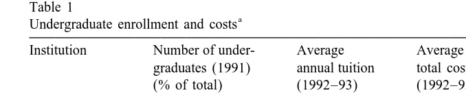
Table 1 reports the costs of different types of colleges. Of the 10 million or so undergraduates in the U.S. each year, about 40% are enrolled in public 4-year colleges. There the average total cost (including room and board) for the 1992–93 academic year was about $6000. About 20% of undergraduates are at private 4-year colleges, where the total cost averaged about $15,000 per year. The
2
Table 1
a
Undergraduate enrollment and costs
Institution Number of under- Average Average annual graduates (1991) annual tuition total costs (% of total) (1992–93) (1992–93) Private, 4 year 2.3 million (19%) $10,393 $15,128 Public, 4 year 4.7 million (38%) 2352 6029 Public, 2 year 5.4 million (44%) 1018 –
a
Notes. Source: DOE (1993). Total costs are in current dollars and include tuition, fees, and room and board assuming full-time enrollment. For public schools tuition is the in-state charge.
remaining undergraduates are mostly at public 2-year colleges, where tuition alone was about $1000 per year.
The fraction of these large costs that households actually pay is hard to estimate, because it varies with the financial-aid package a household receives. Miller and Hexter (1985, 1985a) estimate this fraction for full-time students financially dependent on their families, using the 1983–84 Student Aid Recipient Survey. For the most common aid package, consisting of a Pell grant and state and campus-based aid, middle-income households typically paid at least two-thirds of the total cost of college. Under the next most common package, with a Guaranteed Student Loan instead of state aid, the fraction paid rose to over four-fifths, taking into
3
account the repayment of the loan. For low-income households, the fractions were about one-half and two-thirds, respectively. Miller and Hexter argue that
these [low-income] families have virtually no discretionary income to tap and can rarely call upon savings for [paying this remaining fraction]. Thus we can only speculate that these students are living at a lower standard than was allowed for in their student budget or that they are receiving additional support (from grandparents or other relatives, for example) that is not
4
captured in the need analysis process.
3
Pell grants and GSLs were the most important forms of financial aid. In 1988–89, over 3 million students received Pells, averaging about $1400. About 3.6 million (including graduate students) took out subsidized Stafford loans, averaging about $2600. Many of these students took out the maximum Stafford loan. For them and others ineligible for Staffords, there were also guaranteed PLUS (parent loans to undergraduate students) and SLS (supplemental loans to students) loans. In 1988–89, about 800 thousand students (including graduate students) borrowed an average of about $2600 via SLSs, and 200 thousand borrowed about $3100, on average, via PLUSs (McPherson and Schapiro, 1991). Little is known about other, nonguaranteed loans taken out for college, apart from the self-reported total use of loans described below. About one-third of aid-recipients at public colleges receive only GSLs, so pay 100% of cost (not including the subsidized interest rate). For private colleges, the figure is about one-eighth.
4
The 1986–87 National Postsecondary Student Aid Survey (NPSAS) asked parents themselves how much they contributed to their children’s college costs during the academic year. Choy and Henke (1992) summarize the results for families with dependent undergraduates. Sixty-seven percent of the parents contributed at least some amount, with the average contribution about $3900 (for tuition, housing, and other expenses). On adding the 11% of parents who extended
5
loans to their children, the average conditional contribution was about $4200. On also adding the 83% of parents giving in-kind gifts (e.g., housing and clothing), the average was about $6200. The probability and magnitude of contribution were
6
generally increasing in the income and wealth of the parents. Focusing only on the households with children attending private colleges, the average contribution was about $6500, rising to $8800 on including loans and in-kind gifts. These amounts, usually multiplied by 2 or 4 (for 2- or 4-year colleges, respectively), are
7
substantial relative to typical household income and savings.
According to the NPSAS, of the parents giving gifts (not including in-kind gifts, but including loans), about 80% said they used at least some current income as a source of funds, 65% used some previous savings, 24% used some loans, and 30% used some additional income from increased work. Unfortunately, the dollar amounts used of each source are not available. Still, there are two points worth
8
noting. First, 35% of households did not save in advance at all for college. This fraction rose to about 50% for households of lower income or wealth. Second, the extent to which those using current income are cutting their current consumption, or just diverting other current saving, remains unclear.
Of the parents saving for college, about 47% report they started saving before their child was in junior high, 44% started during junior and senior high, and 10% still waited until after high school ended (20% for poorer families). So, even of the households that save, over half wait until they are at most 6 years from college. And even those starting earlier might not be saving sufficiently. A 1984 Roper poll found that most households that were saving for college were not saving enough to
9
meet at current rates their own stated target for savings by the time of college. In
5
The extent to which the parents will in fact be paid back is unclear.
6
The monotonicity does not hold for loans. See also Churaman (1992) for a multivariate analysis of these gifts.
7
The figures are also important relative to aggregate saving. Gale and Scholz (1994) estimate household contributions for college totaled about $35 billion per year in the mid-1980s. It is interesting that such contributions represent about one-third of the difference between Kotlikoff / Summers and Modigliani in their debate about the relative importance of bequests versus life-cycle savings (Modigliani, 1988).
8
These figures still condition on the parents’ giving. Unconditionally, over one-half of parents with dependent undergraduates did not save at all in advance.
9
sum, it remains unclear whether households have adequate savings and other resources for college, and in particular whether they are substantially cutting their consumption right at the time of college.
2.2. Testing the Life-Cycle Theory
A number of studies have examined the ability of households to smooth their consumption past idiosyncratic fluctuations in their income, especially due to unemployment (e.g., Gruber, 1997). While Cochrane (1991) rejects the hypothesis of complete risk-sharing, Dynarski and Gruber (1997) find quantitatively that households do a relatively good job at consumption-smoothing. The Life-Cycle / Permanent-Income Theory requires that consumption should not fluctuate in particular with predictable (or transitory) changes in income. While the theory is often rejected using aggregate data, aggregation bias can induce spurious excess sensitivity of consumption to income even when there is no such sensitivity in the underlying micro data (Attanasio and Weber, 1995). On the other hand, the results using micro data are more mixed (Deaton, 1992; Browning and Lusardi, 1996). In large part this might be due to the difficulty of isolating the predictable component of income at the micro level. Most studies proceed by instrumenting for income, but since the available instruments are typically poor, their results might be prejudiced against finding significant excess sensitivity. In response, recently a few micro studies have examined specific situations in which it is known in advance that income will change. Shea (1995) looks at the consumption of union members in response to anticipated changes in union contracts, and Souleles (1999) looks at the response of U.S. taxpayers to their income tax refunds, which they had requested in advance as part of their tax returns. Both studies reject the Life-Cycle Theory, with Souleles finding evidence of binding liquidity constraints. (See also Parker, 1989 and Souleles, 1996.) This paper examines a different situation, paying for college, which by contrast avoids complications due to liquidity constraints and changes in marginal utility over the life-cycle.
3. The data
each household-quarter, following the BLS’s classification but excluding educa-tional expenditure. This classification includes many relatively durable and lumpy expenditures which are not readily ‘smoothable’, for instance clothing and repairs. Clothing, in particular, might be less separable from educational expenditure than are other nondurable expenditures, insofar as families send their kids off to college in the fall with new clothing. In response, following Lusardi (1996) such expenditures have been removed to create a subset of nondurables, ‘strictly
10
nondurables’. The average ratio of strictly nondurables to nondurables is about
0.66. A subset of strictly nondurables, food, will also be examined.
The sample is limited to ‘traditional’ collegiate households: households in which there is a child aged 16–24, and no one over 24 in school. Other, less traditional households making college payments are more difficult to analyze. The sample is also limited as usual to households with satisfactory data on consumption. Appendix A provides further details about the data. For traditional collegiate households, the average real COLEXP is about $980 (the median $480) for quarters in which COLEXP is nonzero. These expenditures are most frequent and greatest in magnitude (averaging about $1150) for quarters that include August
11
and September. The large amount of variation in COLEXP should give this
paper’s test of consumption-smoothing more power than many similar tests. Further, since the CEX specializes in recording expenditures, COLEXP is probably better measured than most of the income variables in the CEX used in other tests.
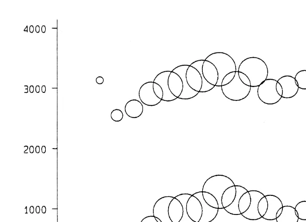
The lower profile in Fig. 1 shows the age distribution of quarterly college expenditure for heads of traditional collegiate households. The frequency (reflected in the size of the bubbles) and magnitude of expenditure are greatest for heads in their middle years (40s and early 50s), the ages at which parents typically send children to college. For comparison, the upper profile in Fig. 1 shows the age distribution of quarterly nondurable consumption for the same household quarters.
10
The major components of strictly nondurables are food, household operations, including monthly utilities and small-scale rentals, transportation fuel and services, including public transportation, personal services, and entertainment services and high-frequency fees.
11
Fig. 1. The age distribution of nondurable and college expenditure. The upper profile shows average nondurable consumption by age, the bottom profile shows average college expenditure by age, both deflated to 1983 $. Ages are assigned to bins of 2 years; only bins with more than 20 observations have their means graphed.
12
This distribution follows a rather similar pattern as that for COLEXP below it. As others have noted (e.g., Carroll and Summers, 1991), the path of nondurable consumption also tracks the path of income with age. But it does not follow that either nondurable or college expenditures are constrained by current income in ways inconsistent with the Life-Cycle Theory. First, progressivity in the financial aid system results in larger college payments when income is larger. Second, other expenditures that are included in nondurables, whether for child-rearing or not, might also naturally be high in the middle years. That is, the marginal utility of consumption might itself be a hump-shaped function of age. Finally, the time path of income might have been sufficiently unpredictable to warrant the observed path of consumption even under the Life-Cycle Theory. In contrast, this paper provides a clean test of whether consumption tracks income by examining an episode
12
during the middle-age years when net income is sharply predictably decreasing because of college expenditures.
4. Econometric specifications
It is convenient to implement the test of consumption-smoothing via an equation interpretable as an Euler equation derived from the Life-Cycle Theory. Following Zeldes (1989) and Lusardi (1996), the equation that governs household i’s change in consumption is specified as
* * *
dC 5Sb time 1b age 1b d(ages 0–15)
i,t11 s 0s s 1 it 2 i,t11
* *
1b d(ages 16–24) 1b d(ages 25–90) 1u , (1)
3 i,t11 4 i,t11 i,t11
where age is the age of the household head in period t, and d(ages 0–15)t t11,
d(ages 16–24) , and d(ages 25–90) record the changes between periods t11
t11 t11
and t in the number of household members less than 16 (e.g., births), between 16 and 24 (inclusive), and greater than 24 (e.g., deaths), respectively. d(ages 16–24) accommodates children leaving the household for college or for other reasons. These demographic variables help control for the most basic changes in the marginal utility of consumption, namely with family size and over time. The full set of dummy variables for time (a separate variable for each month of each year) helps control for seasonality, aggregate shocks, and changes in interest rates across time.
Assuming separability of college expenditures and the rest of nondurable consumption (Feldstein, 1995), the null hypothesis to be tested is that households smooth their consumption even as they pay for college. A natural alternative hypothesis is that households pay for (minus) m% of their college expenditures COLEXP out of current consumption. The generalization of the Euler equation that is estimated is then
* * *
dC 5Sb time 1b age 1b d(ages 0–15)
i,t11 s 0s s 1 it 2 i,t11
* *
1b d(ages 16–24) 1b d(ages 25–90) 1m*COLEXP
3 i,t11 4 i,t11 i,t11
1u , (2)
i,t11
where t11 is the quarter covering the household’s first payments for the fall
semester, with no college payments made in quarter t. The coefficient m then measures the size of the distortion to consumption due to college expenditures. Under the null hypothesis m should be zero. A large negative m would evidence the inadequacy of household resources to smooth consumption in the face of college expenditures. It would count, in particular, as a violation of the Life-Cycle Theory, insofar as COLEXP is a predictable expense by quarter t.
analysis the sample is further restricted to households for whom a CEX reference
quarter t11 can be chosen to include an August or September in which college
expenditures are made. As a result C 2C essentially compares consumption in
t11 t
the fall when paying for college to baseline consumption in the previous summer or late spring. (To avoid any distortion in baseline consumption, the relatively few households making college expenditures in quarter t as well are not included in the sample.) Although college expenditures are from a longer-run point of view endogenous, they have largely been predetermined by this baseline period. Even households with children entering the freshman year of college have usually committed to a particular college and its cost by this time.
The response of consumption in Eq. (2) is net of all the mechanisms available to households to help them smooth their consumption, including loans, contributions from relatives, and other informal resources. There is also a potentially important role for the endogenous choice of college expenditures. Unlike shocks to income resulting from unemployment or disability, for example, college spending is voluntary. Households that foresee their resources will be inadequate for an expensive college can instead choose a less expensive one. Although the longer-run endogeneity of COLEXP and the other consumption-smoothing mechanisms does not vitiate the high-frequency life-cycle test, they can affect the policy implications of the results — especially if households are smoothing their consumption by reducing college expenditures. Unfortunately, the data do not allow one to disentangle the relative importance of the various smoothing mechanisms. But one can nonetheless control for the endogeneity of college expenditures by instrumenting for COLEXP. This will also mitigate any measure-ment error in COLEXP.
It is possible that distortions in consumption due to COLEXPt11do not show up
until later into the academic year, after quarter t11. To test for distortions in the
following winter and spring, the change in consumption over a longer, 6-month
2
where the changes are all over 6 months. Eq. (3) will be estimated for the subset of households used in Eq. (2) that are still present in the data set for an additional
quarter t12. (This is about 60% of the households.) Unfortunately, there are not
enough observations in the data to look further forward in the year.
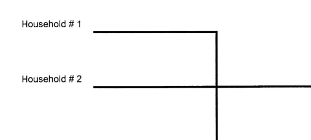
It is interesting to examine consumption before period t as well. To illustrate, Fig. 2 shows two households whose change in consumption between periods t and
t11 is the same, but whose previous paths of consumption are quite different.
Fig. 2. Consumption paths when saving. Household[1 waits to save until period t (crash saving), household[2 starts saving earlier.
suffers a large drop in consumption between periods t21 and t. Household[2 by
contrast started saving earlier, lowering its consumption before period t to avoid a large drop in consumption in period t. To distinguish such households, the
consumption in the fall, quarter t11, will also be examined relative to quarter
t21, the previous spring and winter, using C 2C as the dependent variable:
t11 t21
2 2
* * *
d C 5Sb time 1b age 1b d (ages 0–15)
i,t11 s 0s s 1 it 2 i,t11
2 2
* *
1b d (ages 16–24) 1b d (ages 25–90)
3 i,t11 4 i,t11
1m*COLEXP 1u . (4)
i,t11 i,t11
Again, there is not enough data to look further back in time. And even if there were, inference would be complicated by the fact that college expenditures would
13
less likely be predetermined. Nonetheless, the specifications just described are
sufficient to test whether households have saved enough 6–9 months in advance of the academic year, or have sufficient other resources, to sustain their consumption up to 6 months into the year.
Eqs. (2) to (4) are estimated by OLS, correcting the standard errors for heteroskedasticity. To increase precision, other ‘traditional’ households that do not
make any educational expenditures in any quarter (and whose quarter t11
includes August or September) are added to the sample as a kind of control group, with COLEXP set to zero.
13
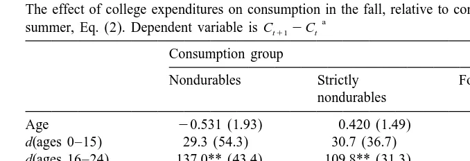
Table 2
The effect of college expenditures on consumption in the fall, relative to consumption in the previous
a
summer, Eq. (2). Dependent variable is Ct112Ct
Consumption group
Nondurables Strictly Food
nondurables
Age 20.531 (1.93) 0.420 (1.49) 0.716 (1.00)
d(ages 0–15) 29.3 (54.3) 30.7 (36.7) 17.4 (24.4) d(ages 16–24) 137.0** (43.4) 109.8** (31.3) 58.2** (24.0) d(ages 25–90) 222.3** (93.2) 201.2** (66.0) 109.4** (50.2) COLEXP 0.083* (0.048) 0.043 (0.028) 0.002 (0.017)
[obs 7109 7200 7200
[(COLEXP.0) 1227 1249 1249
a
Notes. The data are drawn from the CEX from 1980 to 1993. C is real household noneducationals
consumption in quarter s. COLEXP is real total college expenditure in quarter t11. Age is the age of the household head. d(ages 0–15), d(ages 16–24), and d(ages 25–90) record the changes between quarters t11 and t in the number of household members aged less than 16, between 16 and 24, and greater than 24. All regressions also include a full set of month dummy variables. Heteroscedasticity-corrected standard errors in parentheses.
*Significant at the 10% level. **Significant at the 5% level.
5. Results
Table 2 reports the basic results for Eq. (2), for consumption in the fall. For nondurables the coefficient on COLEXP is positive, the unexpected sign, and marginally significant at the 10% level. The coefficients on strictly nondurables and food are smaller and insignificant. Thus, households appear to have enough resources in the fall to maintain their consumption despite large college expendi-tures, consistent with models of consumption-smoothing. As for the demographic control variables, the coefficients on d(ages 16–24) and d(ages 25–90) are positive
and significant, reflecting increased spending with additional household
14
members. Since the demographic coefficients turned out to be similar across
specifications, subsequent tables will not report them. The coefficients on the month dummies, not shown, are together highly significant.
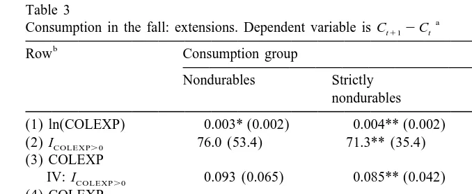
As a check of robustness, Table 3 presents a number of extensions to the basic results. Eq. (2) was first re-estimated in logs. As shown in row (1), again the coefficients on COLEXP are positive, not negative. To guard against measurement
error and endogeneity in the amount expended, COLEXPt11 was replaced by an
indicator variable ICOLEXPt11.0 for making any college expenditures at all. The
resulting coefficients, in row (2), are again all positive, and significant for strictly
14
Table 3
a
Consumption in the fall: extensions. Dependent variable is Ct112Ct b
Row Consumption group
Nondurables Strictly Food
nondurables
(1) ln(COLEXP) 0.003* (0.002) 0.004** (0.002) 0.000 (0.002) (2) ICOLEXP.0 76.0 (53.4) 71.3** (35.4) 27.7 (22.7) (3) COLEXP
IV: ICOLEXP.0 0.093 (0.065) 0.085** (0.042) 0.033 (0.027) (4) COLEXP
IV: STATEEXP 0.038 (0.062) 0.054 (0.040) 0.029 (0.027) (5) COLEXP
(nontrip) 0.029 (0.040) 20.018 (0.022) 20.026 (0.016)
[obs 7109 7200 7200
a
Notes. The data are drawn from the CEX from 1980 to 1993. C is real household noneducationals
consumption in quarter s. COLEXP is real total college expenditure in quarter t11. All regressions also include a full set of month dummy variables and controls for age and changes in family size between quarters t11 and t. Heteroscedasticity-corrected standard errors in parentheses.
b
In row (1), the dependent variable is ln Ct112ln C , the independent variable is ln(COLEXPt 11). In row (2), the independent variable is an indicator for having any college expenditure in t11. In row (3) this indicator variable is used as an instrument for COLEXP. In row (4), real average tuition and fees in the state in which the household resides, STATEEXP, is used as an instrument for COLEXP. In row (5), the dependent variable does not include spending away from home on trips.
* Significant at the 10% level. **Significant at the 5% level.
nondurables though small in magnitude. Households paying for college actually increase their noneducational spending in the fall, by about $75. In row (3) this indicator variable is used as an instrument for COLEXP. Again the coefficients are positive, and significant though small for strictly nondurables. An alternative
instrument for COLEXPt11is average college tuition and fees in the state in which
15
the household resides, STATEEXPt11, which is exogenous to the household. The
results, in row (4), are similar to those using the indicator variable as the instrument, though no longer significant. Both IV results are generally similar to the basic results in Table 2, suggesting that measurement error and endogeneity are not driving the results. The positive coefficients on COLEXP might reflect remaining nonseparabilities between college expenditure and the dependent consumption variables, even for food and strictly nondurables. One possibility is that food and travel spending increases in the fall as parents take their children to college. To investigate this possibility, the consumption categories were re-aggregated without including such spending. The results are in row (5). The
15
The underlying first-stage regression yields COLEXP5283(82)10.30(0.04)*STATEEXP, with the
2
coefficient for nondurables is still positive, but insignificant and smaller than in Table 2. The coefficients for food and strictly nondurables are now negative,
16
though small in magnitude. These extensions confirm the basic result that
households are able to smooth their consumption in the fall. If anything their consumption is slightly increasing, in part due to nonseparabilities.
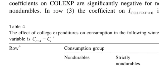
Table 4 reports the results for Eq. (3), for consumption later in the academic year, during the following winter and spring. The basic results appear in row (1). The coefficients on COLEXP are now all negative. While insignificant for nondurables, they are significant for strictly nondurables and food. But again they are rather small in magnitude. The point estimate for strictly nondurables is about
20.07, representing a decline in consumption of only 7 cents for each dollar of
college expenditure. The 95% confidence interval bounds the decline at 13 cents. The second panel of Table 4 explores various extensions. In logs, in row (2), the coefficients on COLEXP are significantly negative for nondurables and strictly
nondurables. In row (3) the coefficient on ICOLEXP.0 implies that household
Table 4
The effect of college expenditures on consumption in the following winter / spring, Eq. (3). Dependent
a
(1) COLEXP 20.073 (0.052) 20.066** (0.031) 20.032** (0.016)
[obs 4175 4216 4216
[(COLEXP.0) 713 728 728
(2) ln(COLEXP) 20.007** (0.002) 20.004** (0.002) 20.002 (0.003) (3) ICOLEXP.0 2222.5** (66.8) 272.4* (44.8) 215.9 (22.4) (4) COLEXP
IV: ICOLEXP.0 20.264** (0.081) 20.086* (0.053) 20.019 (0.032) (5) COLEXP
IV: STATEEXP 20.250** (0.076) 20.101** (0.049) 20.034 (0.029)
a
Notes. The data are drawn from the CEX from 1980 to 1993. C is real household noneducationals
consumption in quarter s. COLEXP is real total college expenditure in quarter t11. All regressions also include a full set of month dummy variables and controls for age and changes in family size between quarters t12 and t. Heteroscedasticity-corrected standard errors in parentheses.
b
Row (1) presents the basic results for consumption in the following winter / spring, relative to the previous summer. In the extensions in the second panel, in row (2) the dependent variable is ln Ct112ln C , the independent variable is ln(COLEXPt 11). In row (3) the independent variable is an indicator for having any college expenditure in t11. In row (4) this indicator variable is used as an instrument for COLEXP. In row (5), real average tuition and fees in the state in which the household resides, STATEEXP, is used as an instrument for COLEXP.
*Significant at the 10% level. **Significant at the 5% level.
16
spending drops by only about $70 in strictly nondurables and another $150 in nondurables. Instrumenting with this indicator variable or with STATEEXP produces similar results, in rows (4) and (5), though somewhat larger in magnitude than the basic results in row (1). In both cases strictly nondurables decline by about 10 cents for each dollar, and nondurables decline by another 15
17
cents. In sum, although there is some delayed decline in consumption in the
following winter and spring, it is not substantial. Households appear to have sufficient resources to do a relatively good job smoothing their consumption well into the academic year. It remains possible that households’ consumption decreases substantially only after the spring. But the original results of Table 2 suggest that consumption does not decrease much further with any new round of college expenditures in the following fall, because such rounds were already included in the sample used for Table 2 for students who were beyond their first
18
year of college.
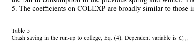
To investigate the possibility of crash saving, Eq. (4) compares consumption in the fall to consumption in the previous spring and winter. The results are in Table 5. The coefficients on COLEXP are broadly similar to those in Table 2 for Eq. (2).
Table 5
Crash saving in the run-up to college, Eq. (4). Dependent variable is Ct112Ct21, consumption in the
a
fall relative to the previous spring and winter Consumption group
Nondurables Strictly Food nondurables
COLEXP 0.092* (0.048) 0.043 (0.031) 0.007 (0.018) [obs 4388 4388 4388
[(COLEXP.0) 783 794 794
a
Notes. The data are drawn from the CEX from 1980 to 1993. C is real household noneducationals
consumption in quarter s. COLEXP is real total college expenditure in quarter t11. All regressions also include a full set of month dummy variables and controls for age and changes in family size between quarters t11 and t21. Heteroscedasticity-corrected standard errors in parentheses.
*Significant at the 10% level.
17
A different response to endogeneity is to compare the consumption of the households with college-age children (whether they make any college expenditures or not) to the consumption of all other households, without college-age children. Eqs. (2) and (3) were re-estimated on this larger sample replacing COLEXP with an indicator variable for having college-age children. In Eq. (2) the indicator was generally negative but not significant, in Eq. (3) the indicator was significantly negative. These results could reflect difficulty smoothing consumption past college expenses. However, they could also reflect a difference in the marginal utility of households with children, one which affects their Euler equation such that their consumption profiles are less steep.
18
This result counts against crash saving, at least crash saving in the previous spring and winter. Insofar as savings are being used to maintain consumption in the fall, this saving appears to be fully underway at least 6 to 9 months in advance.
Of course households can tap many different types of resources in addition to savings to fund college expenditures. Unfortunately, the CEX is not well suited for identifying the resources that are in fact tapped. There is some data available in the first and fourth interviews on household assets and income. Of the assets data, balances in checking and savings accounts are considered the most satisfactory, so it is natural to consider their sum, a measure of liquid assets, and examine the change in liquid assets between interviews four and one. Even though this asset-change variable does not quite match the timing of the consumption-change in Eq. (2), it can still be used as the dependent variable in Eq. (2), keeping the
same independent variables. This yields a coefficient of 20.33 (0.42) on
COLEXP, which, although insignificant, suggests that perhaps as much as
one-19
third of college expenditures might come out of liquid assets. Using instead the
change in income between interviews four and one as the dependent variable yields a coefficient of only 0.02 (1.24) on COLEXP. This insignificant result might be taken as evidence that labor supply does not increase much in order to fund college expenditures. However, the reference period for income covers the entire year preceding the interview; taking the change in annual income between interviews that are only 9 months apart does not match the timing implicit in Eq.
20
(2). In any case, these results must be qualified because the assets and income
data in the CEX are considered less reliable than the expenditure data and are often missing.
The CEX does not contain satisfactory data on other resources that are potentially important in funding college, such as loans, contributions from relatives, and other informal resources. However, such data is not well measured by any household data set. One virtue of the consumption-based approach of this paper is that it does not need explicit and comprehensive measures of household resources to test the null hypothesis of consumption-smoothing. The test implicitly takes into account all of the resources available to the household.
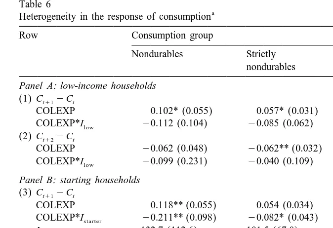
Table 6 investigates whether the main results above vary across certain salient subsets of households. Perhaps households with low levels of income or assets have more trouble smoothing their consumption. Since the assets data is less well
19
Since durable goods are also assets, total consumption (including durables) was also used as the dependent variable in Eq. (3). This led to a coefficient of20.15 (0.11) on COLEXP, about twice the size of the coefficient for nondurables, though insignificant.
20
Table 6
a
Heterogeneity in the response of consumption
Row Consumption group
Nondurables Strictly Food
nondurables Panel A: low-income households
(1) Ct112Ct
COLEXP 0.102* (0.055) 0.057* (0.031) 0.008 (0.020) COLEXP*Ilow 20.112 (0.104) 20.085 (0.062) 20.039 (0.024) (2) Ct122Ct
COLEXP 20.062 (0.048) 20.062** (0.032) 20.038** (0.017) COLEXP*Ilow 20.099 (0.231) 20.040 (0.109) 0.052 (0.055) Panel B: starting households
(3) Ct112Ct
COLEXP 0.118** (0.055) 0.054 (0.034) 0.007 (0.021) COLEXP*Istarter 20.211** (0.098) 20.082* (0.043) 20.016 (0.031) Istarter 132.7 (112.6) 101.5 (67.0) 231.8 (42.6)
[starter 220 224 224
(4) Ct122Ct
COLEXP 20.082 (0.061) 20.056 (0.039) 20.038* (0.020) COLEXP*Istarter 0.070 (0.108) 20.050 (0.049) 0.020 (0.035) Istarter 2136.7 (134.2) 33.0 (82.9) 7.4 (42.6)
[starter 134 137 137
a
Notes. The data are drawn from the CEX from 1980 to 1993. The dependent variable is Ct112Ct
or Ct122C , as indicated. C is real household noneducational consumption in quarter s. COLEXP ist s
real total college expenditure in quarter t11. Ilowis an indicator variable for households with income in the bottom quartile of the income distribution. Istarteris an indicator for households with children first starting college. All regressions also include a full set of month dummy variables and controls for age and changes in family size between the indicated quarters. Heteroscedasticity-corrected standard errors in parentheses.
*Significant at the 10% level. **Significant at the 5% level.
measured, Panel A investigates low income households. An indicator variable Ilow
was created identifying the households with income in the bottom quarter of the income distribution, and interacted with COLEXP. The results for Eq. (2) for the fall appear in row (1). The interaction terms are negative, though not significantly so. For the low-income households, the point estimate for the total response of
strictly nondurables is only 20.028 (50.05720.085), for a consumption decline
by college expenditures than that of higher income households, but not
sig-21,22
nificantly so.
Numerous surveys have suggested that parents know rather little about college costs and financial aid before their children enter college, even as late as the senior year of high school (GAO, 1990). Consequently, it might be that the consumption
23
distortion is greater for households sending children to college for the first time. To investigate this possibility, ideally one would identify households whose first child ever to go to college is entering the first year of college. Unfortunately, this identification is not possible in the CEX, which is not intended to trace family dynamics. Instead one can pick out the households that have some child entering the first year of college, but no other children already in college at the time. (Note that it remains possible that older children have already graduated from college.) About 220 such ‘starting’ households were identified in the sample.
Panel B of Table 6 reports the results on adding separate intercept and interaction terms for these starting households. Row (3) displays the results for Eq. (2), for the fall. The interaction term for nondurables is significantly negative, implying that starting households have more trouble smoothing their consumption.
However, their marginal response is only about 20.09, i.e. starting households’
nondurable consumption drops by less than 10 cents for every additional dollar of college expenditures. The interaction term for strictly nondurables is only marginally significant (at the 10% level). On the other hand, the starters’ intercept term is positive for both nondurables and strictly nondurables, though insignificant. Starting households might be incurring fixed costs that nonstarters no longer
24
incur. Including this effect the total (as opposed to marginal) response of starters’ consumption is about zero at the mean level of COLEXP. The results for Eq. (3) are in row (4). The interaction terms are now all insignificant. However, this might
21
An alternative indicator was created for households with low-education heads. The results are similar to those for low-income households, with the interaction terms negative but insignificant and small.
22
Some studies have found poor people to be less good at consumption-smoothing than others, e.g. Dynarski and Gruber (1997). Some of these findings can be explained by liquidity constraints (Zeldes, 1989; Souleles, 1999), whereas here liquidity constraints are not an issue because net income is declining. Also, the successfulness of smoothing might vary with the context. The poor might do a relatively better job in the case of paying for college because they can foresee the costs in advance and the costs are positively correlated with their resources.
23
The NPSAS survey cited above has some mixed information on this point. Parents’ stated reliance on current income and previous savings is not monotonic in the grade of the student (college freshman to senior and beyond), but does not vary much with it anyway. Use of current income does decrease with the number of other children in college. Use of previous savings increases if there is one other child, though then decreases with more than one child. The largest effect is that parents with other children already in college are much more likely to be saving in general (as opposed to saving for education in particular).
24
be due to the small sample size; only about 130 starting households remain in the sample. In sum, while the consumption of starting households is somewhat more distorted by college expenditures, the size of this extra distortion does not appear to be notably large or persistent.
6. Conclusion
The main finding of this paper is that households sending their children to college appear to do a relatively good job smoothing their consumption well into the academic year, despite large college expenses. Further, households do not sharply cut their consumption in the 6–9 months before the academic year starts. This suggests that whatever saving they do for college has been fully underway at least this many months in advance of their college expenditure. There is, however, some evidence of a delayed decline in consumption in the following winter and spring, and of a decline even in the fall for households with children first beginning college, but the magnitudes of these declines are relatively small. In short the results are broadly consistent with the Life-Cycle Theory, and more generally with any forward-looking theory that requires consumption-smoothing in the face of predictable decreases in income. This consistency is especially noteworthy considering that the test in this paper should be relatively powerful in detecting violations of consumption-smoothing.
It is important to stress, however, that these results do not imply that households find it easy to pay the high cost of college, but only that they are rationally meeting this cost. Even if the slopes of their consumption paths are not much distorted, their levels might have been set rather low in order to accumulate sufficient savings. On the other hand, one might expect households to do a relatively good job smoothing consumption in the particular case of paying for college. They should foresee the potential costs of college many years in
25
advance, and they usually have some access to guaranteed or subsidized loans
26,27
and means-tested financial aid.
This paper might usefully be extended in a number of ways. First, it would be
25
But note that households also know in advance that their income will decline on retirement, and yet there is some concern about the adequacy of their savings for retirement.
26
Though recall that many households are at the borrowing limit of the guaranteed loans. There is also some concern that many households, especially minorities, are ‘unduly’ hesitant to take out loans (Miller and Hexter, 1985, 1985a).
27
interesting to examine the response of consumption over longer periods of time. For instance, given the evidence that households might be saving at least 6–9 months in advance of college, one might try to determine how early they started seriously saving. However, such a longer-run point of view will have to take more explicitly into account the endogeneity of college expenditures. Second, it would be interesting to examine the effect of college expenditures on household portfolios. For example, one might try to better identify the types of assets households draw on to pay for college, especially the role of loans. These extensions will require additional data beyond that available in the CEX. A final extension might investigate more generally the effects on life-cycle savings and consumption of other consumption ‘needs’, such as other aspects of child-rearing or other large expenditures. Do households adequately save in advance of such
28
predictable expenditures, or does their consumption suffer as a result?
Acknowledgements
For helpful comments I thank the editor and two anonymous referees, Orazio Attanasio, Olivier Blanchard, Jerry Hausman, Taejong Kim, Jonathan Parker, Steve Pischke, staff of the Bureau of Labor Statistics, and participants of the MIT and Wharton Macro lunches and the University of Cyprus / Bank of Cyprus Conference on Household Saving and Portfolios. Of course, none of these people are responsible for any errors herein. Financial support from the National Science Foundation is also gratefully acknowledged.
Appendix A
For college students living at home, COLEXP includes all payments for college expenses made by the household. College students living away are not counted by the CEX as part of the ‘consumer unit’, and so are dropped from the data set. Nonetheless, the CEX records the educational expenses incurred by the household for such students. COLEXP includes all such expenses with one exception: cash contributions given directly to a student living away (as opposed to payments made directly to a college or any other third party) are recorded only once, with an annual reference period, and so cannot be used in the quarterly analysis of this
28
29
study. A child is taken to be starting college if it is between 16 and 19 years old,
30
inclusive, and appears to have moved from high school into college in the fall. A
household with such a child is taken to be a ‘starting’ household if it does not have any ‘nonstarting’ members already in college, and does not make any college expenditures in any interview before the fall. (Since the CEX does not keep track of children after leaving the household, one cannot tell whether some older children no longer living with their parents have already graduated from college.) Average state tuition and fees STATEEXP are calculated using data from various issues of the Digest of Education Statistics. STATEEXP is a weighted average across private, public 4-year, and public 2-year institutions. When values are missing in the Digest, they are extrapolated from adjacent years in proportion to the corresponding national growth rate in those years. When the CEX state variable is missing, STATEEXP includes the average expense in the household’s census region instead. If the region variable is also missing, then the average national
31
expense is used instead.
To improve the measurement of consumption, a household was dropped from the sample if there are multiple consumer units in the household, if the household lives in student housing, or if the head’s occupation is farming / fishing. In aggregating expenditures into consumption groups (food, strictly nondurables and nondurables), if any component of a group was topcoded or missing its cost, the whole group was set to missing for the quarter. So too if the household lacks food expenditures in any month of the quarter. If any component of a consumption group was missing its date or dated before the reference period, that group was dropped for all interviews for the household at issue. A nonnegligible number of expenditures are dated in the month of the interview, i.e. the month after the reference period. Following the recommendation of the staff at the BLS, for consistency such expenditures were accrued to the following reference period. If any component of COLEXP was topcoded, COLEXP was set to missing for that
32
quarter. For married households with female respondents, the head of household
29
The main regressions in the text were re-run including these cash contributions (when not flagged) in COLEXP, assuming they were made in quarter t11. The pattern of results and conclusions does not change.
30
Preliminary analysis uncovered some anomalies in the routines the Census Bureau used to clean the variable for the highest grade attended, for teen-aged household members. Census flags, kindly provided by the BLS, were used to undo most of these anomalies, but some might remain. In response, this variable is used only in conjunction with the variables for age and college enrollment.
31
Dropping the observations missing state does not change the conclusions. I thank Taejong Kim for his help with this state tuition data.
32
was taken to be the husband. In computing changes in family size, the artificial changes induced by a member’s moving from age 15 to 16, or from 24 to 25, were suppressed. A handful of other adjustments to the primitive data were made, according to corrections provided in the CEX documentation for various years.
References
Attanasio, O.P., Weber, G., 1995. Is consumption growth consistent with intertemporal optimization? Evidence from the Consumer Expenditure Survey. Journal of Political Economy 103 (6), 1121– 1157.
Browning, M., Lusardi, A., 1996. Household saving: micro theories and micro facts. Journal of Economic Literature 34 (4), 1797–1855.
Carroll, C.D., Summers, L.H., 1991. Consumption growth parallels income growth: some new evidence. In: Bernheim, B.D., Shoven, J.B. (Eds.), National Saving and Economic Performance, Chicago University Press for NBER, Chicago, pp. 305–343.
Case, K.E., McPherson, M.S., 1986. Does need-based student aid discourage saving for college? College Entrance Examination Board, Washington.
Choy, S.P., Henke, R.R., 1992. Parental financial support for undergraduate education. National Center for Education Statistics, U.S. Department of Education, Washington.
Cochrane, J.H., 1991. A simple test of consumption insurance. Journal of Political Economy 99 (5), 957–976.
Churaman, C., 1992. Financing of college education by minority and white families. Journal of Consumer Affairs Winter, 324–350.
Deaton, A., 1992. Understanding Consumption, Oxford University Press, Oxford.
Department of Education, 1993. Digest of Education Statistics. National Center for Education Statistics, Washington.
Dick, A.W., Edlin, A.S., 1997. The implicit taxes from college financial aid. Journal of Public Economics 65 (3), 295–322.
Dynarski, S., Gruber, J., 1997. Can families smooth variable earnings? Brookings Papers on Economic Activity 1, 229–303.
Dynarski, S., 1999. Does aid matter? Measuring the effect of student aid on college attendance and completion. Manuscript, M.I.T.
Edlin, A.S., 1993. Is college financial aid equitable and efficient? Journal of Economic Perspectives Spring, 143–158.
Engelhardt, G.V., 1996. Consumption, down payments, and liquidity constraints. Journal of Money, Credit, and Banking 28 (2), 255–271.
Feldstein, M., 1995. College scholarship rules and private saving. American Economic Review June, 552–566.
Gale, W.G., Scholz, J.K., 1994. Intergenerational transfers and the accumulation of wealth. Journal of Economics Perspectives Fall, 145–160.
General Accounting Office, 1990. Higher education: gaps in parents’ and students’ knowledge of school costs and federal aid. Washington.
Gruber, J., 1997. The consumption smoothing benefits of unemployment insurance. American Economic Review 87 (1), 192–205.
Kane, T.J., 1998. Savings incentives for higher education. National Tax Journal LI (3), 609–620. Kane, T.J., 1994. College entry by blacks since 1970: the role of college costs, family background, and
the returns to education. Journal of Political Economy 102 (5), 878–911.
Lusardi, A., 1996. Permanent income, current income, and consumption: evidence from two panel data sets. Journal of Business and Economic Statistics 14, 81–90.
McPherson, M.S., Schapiro, M.O., 1991. Keeping College Affordable: Government and Educational Opportunity, The Brookings Institution, Washington, DC.
Miller, S.E., Hexter, H., 1985. How Low-income Families Pay For College, American Council on Education, Washington.
Miller, S.E., Hexter, H., 1985a. How Middle-income Families Pay For College, American Council on Education, Washington.
Modigliani, F., 1988. The role of intergenerational transfers and life cycle saving in the accumulation of wealth. Journal of Economic Perspectives Spring, 15–40.
Mumper, M., 1993. The affordability of public higher education: 1970–1990. The Review of Higher Education, 157–180.
Parker, J.A., 1999. The reaction of household consumption to predictable changes in payroll tax rates. American Economic Review, forthcoming.
Roper Organization, 1984. A national study on parental savings for children’s higher education expenses. The National Institute of Independent Colleges and Universities, Washington.
Shea, J., 1995. Union contracts and the life-cycle / permanent-income hypothesis. American Economic Review March, 186–200.
Souleles, N.S., 1996. Consumer response to the Reagan tax cuts. Manuscript, University of Pennsylvania.
Souleles, N.S., 1999. The response of household consumption to income tax refunds. American Economic Review, forthcoming.