T H E J O U R N A L O F H U M A N R E S O U R C E S • 46 • 2
Consequences of Home-Based Work
in the United States, 1980–2000
Gerald S. Oettinger
A B S T R A C T
This study documents the rapid growth in home-based wage and salary employment and the sharp decline in the home-based wage penalty in the United States between 1980 and 2000. These twin patterns, observed for both men and women in most occupation groups, suggest that employer costs of providing home-based work arrangements have decreased. Consis-tent with information technology (IT) advances being an important source of these falling costs, I find that occupation-gender cells that had larger increases in on-the-job IT use also experienced larger increases in the home-based employment share and larger declines in the home-based wage penalty.
I. Introduction
Home-based employment has grown at a rapid rate in the United States in recent decades. According to U.S. census data, the number of home-based workers nearly doubled between 1980 and 2000, growing from less than 2.2 million to nearly 4.2 million, while total employment grew at a much slower pace, from 96.6 million to 128.3 million.1Several forces operating over this time period
poten-tially can explain this dramatic growth in home-based employment. First, the em-ployment share of women grew substantially over this period, and women may value home-based work arrangements more highly than men given the traditional division
Gerald S. Oettinger is an associate professor of economics at the University of Texas at Austin. He thanks the Alfred P. Sloan Foundation for financial support, Anne Golla for valuable research assis-tance, and Karen Conway, Patricia Reagan, and audiences at the IZA/SOLE Transatlantic meetings, the SOLE meetings, and SEA meetings, and UC Santa Barbara for comments. The data used in this article can be obtained beginning October 2011 through September 2014 from Gerald S. Oettinger, Department of Economics, University of Texas, Austin, TX 78712, email: oettinge@eco.utexas.edu.
[Submitted October 2006; accepted January 2010]
of home production tasks within the family. Second, major advances in information and communications technology, which may have reduced the costs of providing home-based work arrangements, also occurred during these years. Finally, shifts in the occupational mix of the U.S. labor force over this period may have favored growth in home-based work.
The few existing empirical studies of home-based employment (Kraut and Grambsch 1987; Kraut 1988; Presser and Bamberger 1993; Edwards and Field-Hendry 2001, 2002; Pabilonia 2005; Schroeder and Warren 2005) all have analyzed its determinants or wage consequences at a point in time. While valuable, these studies offer little insight into why home-based employment has expanded so rapidly in recent years. The present paper begins to fill this gap by using data from the Public Use Micro Samples (PUMS) of the 1980, 1990, and 2000 U.S. Censuses to analyze in detail both the recent growth in home-based wage and salary employment and the contemporaneous changes in the wages of home-based employees relative to onsite workers.
I find that the rapid growth in home-based wage and salary employment was accompanied by a dramatic decline in the wage penalty associated with home-based work, from roughly 30 log points in 1980 to approximately zero in 2000. More disaggregated analyses reveal that based employment shares rose and home-based wage penalties declined in almost all occupation categories, for both men and women, and that only small fractions of the growth in the overall home-based em-ployment share and the decline in the average home-based wage penalty can be explained by compositional shifts favoring occupation groups with high propensities toward and low-wage penalties from home-based work. These results suggest that broad-based reductions in employer costs of providing home-based work arrange-ments have been the predominant force behind the growth in home-based employ-ment since 1980.
I then investigate whether the data are consistent with advances in information technology (IT) being a major source of these decreasing costs. If IT advances played an important role, gender-occupation categories that saw greater growth in on-the-job IT use should have experienced larger increases in home-based employ-ment shares and larger declines in home-based wage penalties. I use data from Current Population Survey (CPS) supplements to construct measures of IT use within gender⳯occupation⳯year cells and find evidence consistent with these hypotheses. I also use data from the Occupational Information Network (O*NET)—the database that replaced the Dictionary of Occupational Titles (DOT)—to compute, for each gender-occupation category, the fraction of jobs requiring less than weekly face-to-face discussion with customers or coworkers. I find some evidence that, for a given level of growth in on-the-job IT use, home-based employment shares grew more in gender-occupation cells with a higher fraction of jobs requiring less than weekly face-to-face discussion. However, I find no evidence that an analogous interaction effect helps account for the pattern of decline in home-based wage penalties.
the empirical analyses to be undertaken. Section IV presents the results of the em-pirical analyses and Section V concludes.
II. Data
The empirical analyses use data from the 5 percent Public Use Mi-crodata Samples (PUMS) of the U.S. Census of Population for 1980, 1990, and 2000. In each of these years, the census long form contained a question about the method of transportation used to get to work on the most days in the previous week. Responses to this question were obtained for all individuals who were aged 16 or older and were employed in the previous week. I classify employed individuals who select the response “worked at home” as home-based workers and classify all others as onsite workers. Since only individuals whomainlywork at home are counted as home-based, the frequency of home-based employment in the census data is a con-servative lower bound on the fraction of workers who do anywork at home.2
For each census year, I construct analysis samples by first selecting all households that contain one or more home-based workers and a random 1 percent sample of households that contain zero home-based workers.3 From this set of households I
keep all individuals aged 25–64 who were employed in paid civilian jobs in the previous week. In addition, as is discussed further below, I drop the self-employed and limit attention to wage and salary workers in most of the analyses. Thus, the study primarily focuses on prime-age, civilian, wage-and-salary workers.
For all analyses of wages, I compute the hourly wage as wage and salary income in the previous calendar year divided by the product of weeks worked in the previous calendar year and usual hours worked per week. Reported wage and salary income was topcoded at $75,000, $140,000, and $175,000 in the 1980, 1990, and 2000 censuses, respectively.4For observations with topcoded wage and salary income, I
impute annual wage and salary income as 1.5 times the topcode income level before computing the hourly wage. I convert the nominal hourly wage in all census years to real 1999 dollars using the CPI for all urban consumers. Because reported wage and salary income corresponds to the previous calendar year, some or all of this income may have been earned on a different job than the one held on the census date (April 1), from which home-based work status is determined. Thus, home-based work status (and other job characteristics) may be measured with some error with respect to the wage calculated from prior year earnings. This potential misclassifi-cation of home-based work status could cause bias in cross-section estimates, but it will affect over time comparisons only if the durability of home-based jobs has
2. In fact, data from the May 2001 Current Population Survey indicate that 19.8 million workers didsome work at home at least once a week. This number is taken from the U.S. Bureau of Labor Statistics news release “Work at Home in 2001” available at http://www.bls.gov/news.release/homey.nr0.htm.
3. I adjust the census-provided sample weights to account for the differential probabilities of sample inclusion for individuals from households with home-based workers and individuals from households with-out home-based workers and I use these adjusted weights in all of the empirical analyses.
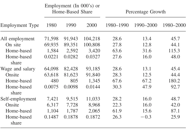
Table 1
Employment Levels, Home-Based Employment Shares, and Their Growth Rates, for Paid Civilian Workers Aged 25–64, by Employment Type and Year
Employment (In 000’s) or
Home-Based Share Percentage Growth
Employment Type 1980 1990 2000 1980–1990 1990–2000 1980–2000
All employment 71,598 91,943 104,218 28.6 13.4 45.7 On site 69,935 89,351 100,808 27.8 12.8 44.1 Home-based 1,584 2,592 3,420 63.6 31.6 115.3 Home-based
share
0.0221 0.0282 0.0327 27.6 16.0 48.0
Wage and salary 64,098 82,428 93,185 28.6 13.1 45.4 Onsite 63,618 81,623 91,840 28.3 12.5 44.4 Home-based 480 805 1,345 67.6 67.2 180.2 Home-based
share
0.0075 0.0098 0.0144 30.3 47.9 92.7
Self-employment 7,421 9,515 11,033 28.2 16.0 48.7 Onsite 6,317 7,728 8,968 22.3 16.0 42.0 Home-based 1,104 1,787 2,065 61.9 15.6 87.1 Home-based
share
0.1487 0.1878 0.1872 26.3 ⳮ0.3 25.9
Note: Data come from the 5 percent PUMS of the U.S. Census of Population for 1980, 1990, and 2000. The samples consist of individuals aged 25–64 who worked for pay in civilian jobs in the week prior to the census. The samples include all such individuals from households containing at least one home-based worker and all such individuals from a 1 percent random sample of households containing no home-based workers. The results in this and all other tables use the census sample weights, adjusted for the differential probabilities of sample inclusion for individuals from households with and without any home-based work-ers. Self-employment includes self-employed individuals working in both incorporated and unincorporated businesses.
changed substantially over time. However, the available evidence for all jobs does not indicate any large secular trend in job stability.5
Table 1 documents the rapid growth in home-based employment among paid ci-vilian workers aged 25–64. The top panel of the table shows that employment of all home-based workers more than doubled between 1980 and 2000 (from 1.58 million to 3.42 million) while employment of all onsite workers grew by only 44.1 percent (from almost 70 million to around 100.8 million) over the same period.6The
remaining panels highlight the substantial differences in both the level and the growth of home-based employment between wage and salary employees and the
self-employed. Home-based employment has been very uncommon among wage and salary workers but has grown extremely rapidly in recent decades, dwarfing the growth rate of onsite wage and salary employment. In contrast, home-based self-employment has been much more common but has grown at a considerably slower rate in recent decades.
For several reasons, I restrict attention to home-based wage and salary workers in the rest of the paper. First, the different growth trends for home-based wage and salary employment and home-based self-employment suggests that different forces may have driven the growth in these two employment sectors, which in turn suggests that the two sectors should be analyzed separately. Furthermore, within the concep-tual framework presented below, an analysis of changes in the relative wages of home-based workers can shed light on the causes of growth in home-based work. This framework assumes that (i) each worker faces a parametric market wage given her skills, (ii) observed average hourly earnings are a good proxy for this (constant) marginal wage, and (iii) there exists a market compensating differential for the non-wage job attribute “home-basedness.” These assumptions seem reasonable for non-wage and salary workers but not for the self-employed. By dropping the self-employed I avoid these difficulties, albeit at the cost of ignoring a quantitatively important com-ponent of total home-based employment.
III. Theoretical Considerations and Empirical Strategy
“Home-basedness” is a job attribute that is worth more to workers with high opportunity costs of spending time away from home and that is less costly to provide on jobs where in-person interaction with coworkers, supervisors, or phys-ically immobile capital inputs is not required. In equilibrium, a market compensating differential for “home-basedness” will equalize the number of workers seeking home-based jobs and the number of home-based jobs offered by employers, and will match workers who value this attribute most with employers who can provide it at lowest cost.7A wage penalty for home-based work will exist in equilibrium if and
only if “home-basedness” is valuable to the marginal home-based worker and is costly to provide for the marginal employer offering home-based work.8
The growth over time in the home-based share of wage and salary employment could be explained either by rising worker valuations for such work arrangements (an outward shift in the relative supply of labor to home-based jobs) or by falling employer costs of offering them (an outward shift in the relative demand for labor in home-based jobs). Rising female labor force participation or changes in prefer-ences or income within demographic groups may have increased worker valuations
7. Rosen (1986) surveys the theory of compensating differentials in detail. A large empirical literature attempts to measure compensating differentials for various job attributes including fatality risk (Thaler and Rosen 1975), unemployment risk (Abowd and Ashenfelter 1981; Topel 1984), shift work (Kostiuk 1990), and employer-provided health insurance benefits (Olson 2002).
of home-based work in recent decades. Over this same period, IT advances may have reduced employers’ nonwage costs of providing home-based work arrange-ments. Fortunately, the observed change in the home-based wage penalty (or pre-mium) over this time period can provide evidence on the relative importance of these competing explanations. In particular, if rising worker valuations for home-based work were the dominant factor, the home-home-based wage penalty should have increased in recent decades. In contrast, if decreasing employer costs of offering home-based jobs were the major driving force, the home-based wage penalty should have fallen over time.
To provide initial evidence on whether the growth in home-based employment is mainly due to rising worker valuations for such work arrangements or falling em-ployer costs of providing them, I estimate log wage regressions of the form
lnW ⳱X  Ⳮ␦ H Ⳮε ,
(1) ist ist st st ist ist
whereiindexes individuals, sindexes gender,tindexes census year,Xis a vector of human capital variables, and His a dummy for home-based employment status. This specification allows the penalty for home-based work (and the returns to ob-served human capital) to vary by gender and year, and the question of interest is how the estimated (male and female) home-based wage penalties,␦stˆ , have changed over time.
The empirical specification in Equation 1 estimates a common home-based wage penalty for all occupations within each gender-year sample. This restriction is un-palatable if, as seems likely, home-based work arrangements can be provided at much lower cost for some jobs than for others. Moreover, if such cost heterogeneity exists, any changes in the aggregate home-based penalty estimated by Equation 1 will confound the effects of shifts in the occupational composition of home-based employment with changes in home-based wage penalties within occupations. Simi-larly, shifts in the occupational composition of the overall labor force might explain some of the growth in home-based employment documented earlier. To address these questions, I next estimate models of the form
20
j
lnW ⳱X  Ⳮ ␦ D H Ⳮε , (2) ist ist st
兺
jst ist ist istj⳱1
where Dj is a dummy that equals 1 if the sample individual is employed in oc-ist
cupation category j and the other variables are defined as in Equation 1.9 This
specification estimates 20 occupation-specific home-based wage penalties in each gender-year sample and allows Oaxaca-type decompositions to be used to assess the role of compositional shifts in explaining changes in the aggregate home-based wage penalty. Analogously, I tabulate home-based employment shares for each of the 20 occupation groups in each gender-year sample and use decomposition methods to evaluate the extent to which compositional shifts explain changes in the aggregate home-based employment share.
Finally, I examine whether the variation in home-based employment shares and home-based wage penalties across gender⳯occupation⳯year cells can be partly explained by across-cell variation in on-the-job IT use and whether this relationship is moderated by how frequently face-to-face discussion with coworkers or customers is required on the job. This analysis is motivated by the observation that home-based employment shares (wage penalties) should have increased (decreased) more in gen-der-occupation cells where on-the-job IT use grew more—ifthis greater utilization of IT substantially lowered employer costs of offering home-based jobs. To test this hypothesis, I estimate variants of the model
y ⳱␥IT Ⳮ␥(IT ⳯LessThanWeeklyDiscussion )Ⳮ ⳭⳭu ,
(3) jst 1 jst 2 jst js js t jst
where jindexes occupation group, s indexes gender, t indexes census year,yjst is either the cell-specific home-based employment share or cell-specific home-based wage penalty, ITjst is a gender⳯occupation⳯year-specific rate of on-the-job IT use10, and LessThanWeeklyDiscussion is the fraction of jobs in each
gen-js
der⳯occupation cell that require less than weekly face-to-face discussion with
co-workers or customers.11
If more IT-intensive jobs can be performed from home more cheaply, then higher on-the-job IT use should be associated with higher (lower) home-based employment shares (wage penalties) and I should find ␥ˆ1⬎0. If this effect is stronger for jobs that require less face-to-face interaction, then I also should find␥ˆ2⬎0. Note that I look for these relationships of interest after controlling for both fixed gender-occu-pation effects and fixed time effects, factors that almost certainly account for much of the variation in home-based employment shares and home-based wage penalties.
IV. Empirical Analyses
A. Descriptive Statistics
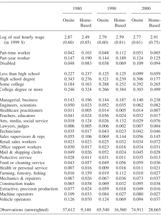
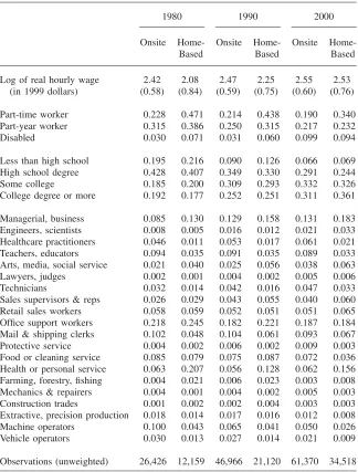
Before reporting estimates of the wage penalty on home-based jobs, Tables 2A and 2B present, for males and females respectively, descriptive statistics on the wages and human capital attributes of onsite and home-based workers between 1980 and 2000. The samples of wage and salary workers are the same as in Table 1, but with the added restriction that only observations with real hourly wages between $1 and $150 are included. The relative wage gains made by home-based workers over these 20 years are striking. In 1980, the mean log real wage of home-based workers was far below that of onsite workers, for both men and women. By 2000, however,
10. This variable is computed using micro data on civilian wage and salary workers aged 25–64 from special CPS supplements in October 1984, September 1993, and September 2001. Details on how this variable is constructed are provided in Section IV below.
Table 2A
Sample Means (Standard Deviations) for Key Variables for Male Wage and Salary Workers Aged 25–64, by Year and Onsite/Home-Based Status
1980 1990 2000
Onsite Home-Based
Onsite Home-Based
Onsite Home-Based
Log of real hourly wage 2.87 2.49 2.79 2.59 2.77 2.91 (in 1999 $) (0.60) (0.85) (0.60) (0.81) (0.61) (0.75)
Part-time worker 0.042 0.103 0.048 0.112 0.051 0.085 Part-year worker 0.147 0.190 0.144 0.189 0.124 0.125 Disabled 0.048 0.083 0.038 0.069 0.109 0.094
Less than high school 0.227 0.237 0.125 0.125 0.099 0.059 High school degree 0.343 0.276 0.321 0.239 0.306 0.177 Some college 0.184 0.163 0.288 0.252 0.292 0.265 College degree or more 0.246 0.324 0.266 0.384 0.303 0.499
Managerial, business 0.143 0.196 0.144 0.187 0.140 0.238 Engineers, scientists 0.050 0.023 0.052 0.035 0.062 0.082 Healthcare practitioners 0.011 0.005 0.014 0.005 0.014 0.007 Teachers, educators 0.041 0.024 0.036 0.024 0.032 0.017 Arts, media, social service 0.018 0.124 0.026 0.132 0.029 0.076 Lawyers, judges 0.006 0.005 0.006 0.002 0.007 0.004 Technicians 0.035 0.017 0.043 0.023 0.042 0.046 Sales supervisors & reps 0.055 0.106 0.069 0.144 0.056 0.145 Retail sales workers 0.023 0.023 0.025 0.032 0.034 0.072 Office support workers 0.030 0.017 0.023 0.016 0.034 0.031 Mail & shipping clerks 0.049 0.026 0.052 0.024 0.045 0.028 Protective service 0.028 0.011 0.031 0.011 0.035 0.013 Food or cleaning service 0.043 0.057 0.049 0.056 0.059 0.036 Health or personal service 0.007 0.016 0.009 0.016 0.011 0.021 Farming, forestry, fishing 0.016 0.159 0.019 0.112 0.010 0.027 Mechanics & repairers 0.067 0.026 0.067 0.036 0.073 0.037 Construction trades 0.065 0.038 0.069 0.032 0.095 0.038 Extractive, precision production 0.077 0.024 0.059 0.018 0.049 0.016 Machine operators 0.109 0.033 0.084 0.027 0.080 0.027 Vehicle operators 0.126 0.070 0.124 0.069 0.094 0.037
Observations (unweighted) 37,612 9,140 65,540 16,560 74,911 28,665
Table 2B
Sample Means (Standard Deviations) for Key Variables for Female Wage and Salary Workers Aged 25–64, by Year and Onsite/Home-Based Status
1980 1990 2000
Onsite Home-Based
Onsite Home-Based
Onsite Home-Based
Log of real hourly wage 2.42 2.08 2.47 2.25 2.55 2.53 (in 1999 dollars) (0.58) (0.84) (0.59) (0.75) (0.60) (0.76)
Part-time worker 0.228 0.471 0.214 0.438 0.190 0.340 Part-year worker 0.315 0.386 0.250 0.315 0.217 0.232 Disabled 0.030 0.071 0.031 0.060 0.099 0.094
Less than high school 0.195 0.216 0.090 0.126 0.066 0.069 High school degree 0.428 0.407 0.349 0.330 0.291 0.244 Some college 0.185 0.200 0.309 0.293 0.332 0.326 College degree or more 0.192 0.177 0.252 0.251 0.311 0.361
Managerial, business 0.085 0.130 0.129 0.158 0.131 0.183 Engineers, scientists 0.008 0.005 0.016 0.012 0.021 0.033 Healthcare practitioners 0.046 0.011 0.053 0.017 0.061 0.021 Teachers, educators 0.094 0.035 0.091 0.035 0.089 0.033 Arts, media, social service 0.021 0.040 0.025 0.056 0.038 0.063 Lawyers, judges 0.002 0.001 0.004 0.002 0.005 0.006 Technicians 0.032 0.014 0.042 0.016 0.047 0.033 Sales supervisors & reps 0.026 0.029 0.043 0.055 0.040 0.060 Retail sales workers 0.058 0.059 0.052 0.051 0.051 0.065 Office support workers 0.218 0.245 0.182 0.221 0.187 0.184 Mail & shipping clerks 0.102 0.048 0.104 0.061 0.093 0.067 Protective service 0.004 0.002 0.006 0.002 0.009 0.003 Food or cleaning service 0.085 0.079 0.075 0.087 0.072 0.036 Health or personal service 0.063 0.207 0.056 0.128 0.062 0.156 Farming, forestry, fishing 0.004 0.021 0.006 0.023 0.003 0.008 Mechanics & repairers 0.004 0.001 0.004 0.002 0.005 0.003 Construction trades 0.001 0.002 0.002 0.004 0.003 0.003 Extractive, precision production 0.018 0.014 0.017 0.016 0.012 0.008 Machine operators 0.100 0.043 0.065 0.041 0.050 0.026 Vehicle operators 0.030 0.013 0.027 0.014 0.021 0.009
Observations (unweighted) 26,426 12,159 46,966 21,120 61,370 34,518
female home-based workers had achieved wage parity with their onsite counterparts and male home-based workers had actually surpassed their onsite counterparts.
The relative wage gains made by home-based workers were accompanied by relative gains in labor force attachment and educational attainment. In 1980, home-based workers were much more likely than onsite workers to work on a part-time or part-year basis or to have a disability; by 2000, these gaps had diminished sub-stantially and, in some cases, disappeared.12With respect to education, home-based
workers and onsite workers had similar attainments in 1980, but home-based workers had an advantage by 2000 and, for males, the gap was quite large.
The final panels of Tables 2A and 2B report occupational distributions, by gender and home-based work status, between 1980 and 2000. Not surprisingly, the occu-pational distributions differ substantially between males and females (holding home-based work status constant) and between onsite and home-home-based workers (holding gender constant) in all years.13Perusal of the home-based worker occupational
dis-tributions reveals that home-based employment shifted from farming and (some) service jobs toward managerial, scientific, and sales jobs over the sample period.
B. Estimates of the Wage Penalty on Home-Based Jobs, 1980–2000
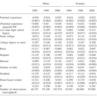
Clearly, one must adjust for the large differences in skills and labor force attachment between onsite and based workers when attempting to measure the home-based wage penalty in each gender-year sample. To this end, I report OLS estimates of Model 1 in Table 3.14I do not discuss the estimated coefficients on the covariates
other than home-based work status, which generally have the expected signs and magnitudes.15Interestingly, the estimated male and female home-based wage
pen-alties differ little in each census year after controlling for observable human capital. More importantly, both male and female home-based wage penalties have fallen
12. Reportedlevelsof disability rose in 2000 for all workers, irrespective of home-based status or sex, because of a change in the wording of the census question about disability status. However, therelative frequency of disability among home-based workers declined sharply in 2000.
13. In unreported tabulations using the complete 5 percent sample from the 2000 census, I also find large gender differences in the detailed occupational distributionswithinthe 20 occupational groups defined in Tables 2A and 2B. This evidence that men and women tend to work in different specific occupations within occupational categories provides support for estimating the empirical models separately by gender. 14. OLS estimates of␦stwill be consistent for the true market compensating differential for home-based employment only if the unobserved wage component is uncorrelated with home-based work status. If workers with high unobserved skills “buy” more desirable job attributes (as suggested by Brown 1980) and if working from home is desirable, the unobserved wage component and home-based work status will tend to be positively correlated. On the other hand, working from home eliminates fixed commuting costs (as emphasized by Edwards and Field-Hendry 2001, 2002), which is more likely to alter work decisions of low-wage workers and which therefore will tend to induce a negative correlation between the unobserved wage component and home-based work status. Thus, the sign of any bias in cross-section estimates of the based work compensating differential is unclear a priori. Still, changes over time in estimated home-based wage penalties may partly reflect changes in unobserved skills of home-home-based workers (relative to onsite workers) rather than pure changes in the implicit price of “home-basedness” for a worker of fixed skill. However, this potential confound is likely to be less severe in the analyses that estimate separate home-based wage penalties for each gender-occupation group.
Table 3
Log wage regressions for wage and salary workers aged 25–64, separately by year and gender, allowing for a homogeneous wage penalty for home-based work
Males Females
1980 1990 2000 1980 1990 2000
Potential experience 0.036 0.034 0.025 0.018 0.020 0.022 (0.002) (0.002) (0.002) (0.002) (0.002) (0.002) (Potential experience
squared)/100
ⳮ0.056 ⳮ0.05 ⳮ0.038 ⳮ0.032 ⳮ0.032 ⳮ0.036
(0.003) (0.003) (0.003) (0.004) (0.004) (0.003) Less than high school
degree
ⳮ0.145 ⳮ0.205 ⳮ0.162 ⳮ0.064 ⳮ0.084 ⳮ0.131
(0.012) (0.014) (0.015) (0.015) (0.017) (0.019) Some college 0.074 0.105 0.122 0.073 0.114 0.129
(0.012) (0.010) (0.010) (0.013) (0.011) (0.010) College degree or more 0.287 0.346 0.330 0.259 0.367 0.398
(0.014) (0.013) (0.013) (0.017) (0.014) (0.013) Black ⳮ0.131 ⳮ0.087 ⳮ0.060 0.062 0.022 0.007
(0.016) (0.015) (0.014) (0.016) (0.015) (0.013) Hispanic ⳮ0.110 ⳮ0.106 ⳮ0.109 0.004 ⳮ0.005 ⳮ0.046
(0.018) (0.015) (0.014) (0.022) (0.021) (0.016) Married 0.099 0.119 0.136 ⳮ0.017 ⳮ0.021 0.001
(0.012) (0.010) (0.010) (0.010) (0.009) (0.008) Number of kids 0.016 0.010 0.010 ⳮ0.036 ⳮ0.031 ⳮ0.017
(0.004) (0.004) (0.004) (0.004) (0.004) (0.004) Disabled ⳮ0.170 ⳮ0.147 ⳮ0.059 ⳮ0.117 ⳮ0.112 ⳮ0.034
(0.022) (0.022) (0.013) (0.031) (0.029) (0.014) Home-based worker ⳮ0.314 ⳮ0.180 0.015 ⳮ0.290 ⳮ0.170 ⳮ0.030
(0.012) (0.010) (0.007) (0.011) (0.009) (0.007) R2 0.224 0.296 0.281 0.198 0.267 0.281
Number of observations (unweighted)
46,752 82,100 103,576 38,585 68,086 95,888
Note: Heteroskedasticity-robust standard errors are shown in parentheses. The estimates use the adjusted census sample weights that account for the varying probability of sample inclusion across observations. All specifications also include dummies for seven industries, 19 occupations, part-time work status, and part-year work status.
arrange-ments may vary with job tasks and since workers’ valuations of working at home may vary with full income or personal attributes, it is in fact likely that both home-based employment shares and home-home-based wage penalties vary a lot across occu-pations. Thus, it is important to investigate whether such heterogeneity is present in the data.
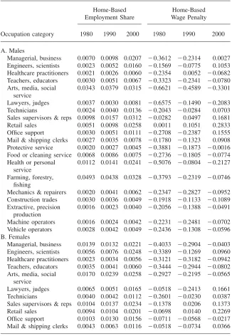
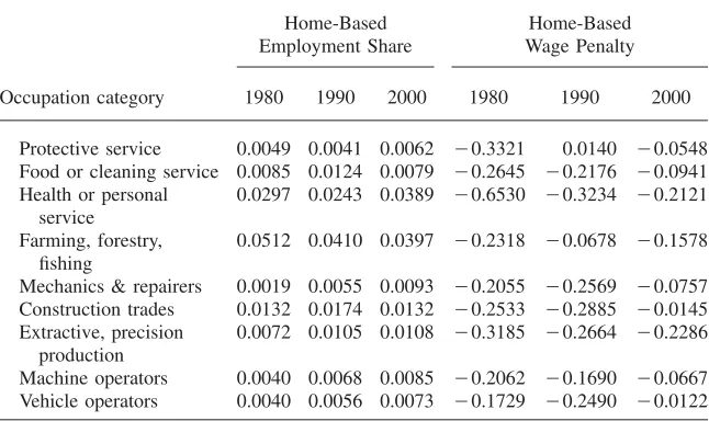
C. Occupational Heterogeneity in Home-Based Employment Shares and Wage Penalties
Table 4 presents estimates of occupation-specific home-based employment shares and occupation-specific home-based wage penalties for all six gender-year samples using 20 mutually exclusive and exhaustive occupation categories. The hypothesis that the shares of home-based workers are equal across occupation groups can be rejected at conventional significance levels in all gender-year samples. In most oc-cupation-year cells, women were more likely to hold home-based jobs than men, reflecting gender differences either in preferences or in detailed occupational affili-ation within occupaffili-ation categories. In nearly all gender-occupaffili-ation cells, the home-based employment share grew between 1980 and 2000, although the pace of this growth varied substantially across cells.
Occupation-specific home-based wage penalties are obtained by estimating the log wage regression in Equation 2. To save space, the table reports point estimates only for the occupation⳯home-based work status interaction terms and does not report standard errors.16As was true for home-based employment shares, the hypothesis
that the wage penalties on home-based jobs were identical across occupation cate-gories is soundly rejected in every gender-year sample. Wage penalties for home-based employment shrank over time in the vast majority of gender-occupation cate-gories; in 1980, these penalties were large in most categories but, by the year 2000, home-based workers in a few gender-occupation groups (for example, sales workers and engineers of both sexes) actually earned substantially more on average than observationally equivalent onsite workers.
Given that home-based employment shares (wage penalties) varied a lot across occupations, it is reasonable to ask whether shifts in the occupational composition of overall (home-based) employment can explain much of the increase (decrease) in the aggregate home-based employment share (wage penalty). To answer these ques-tions, I use standard decomposition techniques. LetHstdenote the home-based em-ployment share among all wage and salary workers aged 25–64 of gendersat date . Let denote the analogous home-based employment share within occupation t Hjst
group j. Then Hst⳱
兺
j20⳱1f Hjst jst, where fjst is occupation group j’s share in total wage and salary employment of gendersat datet. The change in the average home-based employment share of gendersbetween datestandcan be decomposed as20 20
HjsⳭHjst fjsⳭfjst
H ⳮH ⳱ (f ⳮf ) Ⳮ (H ⳮH ).
(4) s st
兺
js jst冢
冣 冢
兺
冣
js jst2 2
j⳱1 j⳱1
The first term in Equation 4 is the part of the change in the aggregate home-based share of gendersthat is explained by changes over time in the occupational
Table 4
Actual home-based employment shares and estimated home-based wage penalties, by occupation-gender category and year
Home-Based Employment Share
Home-Based Wage Penalty
Occupation category 1980 1990 2000 1980 1990 2000
A. Males
Managerial, business 0.0070 0.0098 0.0207 ⳮ0.3612 ⳮ0.2314 0.0027
Engineers, scientists 0.0023 0.0052 0.0160 ⳮ0.1569 ⳮ0.0775 0.1053
Healthcare practitioners 0.0021 0.0026 0.0060 ⳮ0.2354 0.0052 ⳮ0.0682
Teachers, educators 0.0030 0.0051 0.0067 ⳮ0.3323 ⳮ0.2341 ⳮ0.0780
Arts, media, social service
0.0343 0.0379 0.0315 ⳮ0.6621 ⳮ0.4589 ⳮ0.3301
Lawyers, judges 0.0037 0.0030 0.0081 ⳮ0.6575 ⳮ0.1490 ⳮ0.2083
Technicians 0.0024 0.0040 0.0136 ⳮ0.2043 ⳮ0.0284 0.0703
Sales supervisors & reps 0.0098 0.0157 0.0312 ⳮ0.0282 0.0497 0.1681
Retail sales 0.0051 0.0098 0.0258 0.0011 0.1051 0.2833 Office support 0.0030 0.0051 0.0111 ⳮ0.2708 ⳮ0.2387 0.1555
Mail & shipping clerks 0.0027 0.0035 0.0078 ⳮ0.1780 ⳮ0.1323 0.0908
Protective service 0.0020 0.0027 0.0045 ⳮ0.3881 ⳮ0.1873 ⳮ0.0016
Food or cleaning service 0.0068 0.0086 0.0075 ⳮ0.2736 ⳮ0.1805 ⳮ0.0774
Health or personal service
0.0112 0.0141 0.0241 ⳮ0.5076 ⳮ0.0804 ⳮ0.2127
Farming, forestry, fishing
0.0493 0.0438 0.0328 ⳮ0.3793 ⳮ0.2319 ⳮ0.0746
Mechanics & repairers 0.0020 0.0041 0.0062 ⳮ0.2347 ⳮ0.2827 ⳮ0.0952
Construction trades 0.0030 0.0036 0.0049 ⳮ0.1918 ⳮ0.1133 ⳮ0.1089
Extractive, precision production
0.0016 0.0023 0.0040 ⳮ0.2056 ⳮ0.1388 ⳮ0.0491
Machine operators 0.0016 0.0024 0.0042 ⳮ0.2231 ⳮ0.2481 ⳮ0.0702
Vehicle operators 0.0028 0.0042 0.0049 ⳮ0.2436 ⳮ0.1308 ⳮ0.0596
B. Females
Managerial, business 0.0139 0.0132 0.0221 ⳮ0.4033 ⳮ0.2904 ⳮ0.0403
Engineers, scientists 0.0056 0.0076 0.0248 ⳮ0.3389 ⳮ0.1269 0.0960
Healthcare practitioners 0.0023 0.0034 0.0056 ⳮ0.3121 ⳮ0.3182 ⳮ0.0942
Teachers, educators 0.0035 0.0041 0.0060 ⳮ0.3444 ⳮ0.2944 ⳮ0.0802
Arts, media, social service
0.0170 0.0239 0.0258 ⳮ0.2927 ⳮ0.2195 ⳮ0.0565
Lawyers, judges 0.0065 0.0051 0.0165 ⳮ0.0518 ⳮ0.2413 0.1661
Technicians 0.0040 0.0042 0.0112 ⳮ0.2601 ⳮ0.0230 0.0387
Sales supervisors & reps 0.0104 0.0137 0.0234 ⳮ0.1378 0.0206 0.1373
Retail sales 0.0094 0.0104 0.0201 ⳮ0.0698 0.0140 0.2269
Office support 0.0103 0.0130 0.0156 ⳮ0.0711 ⳮ0.0568 ⳮ0.0217
Mail & shipping clerks 0.0043 0.0063 0.0116 ⳮ0.0518 ⳮ0.0734 0.0366
Table 4(continued)
Home-Based Employment Share
Home-Based Wage Penalty
Occupation category 1980 1990 2000 1980 1990 2000
Protective service 0.0049 0.0041 0.0062 ⳮ0.3321 0.0140 ⳮ0.0548
Food or cleaning service 0.0085 0.0124 0.0079 ⳮ0.2645 ⳮ0.2176 ⳮ0.0941
Health or personal service
0.0297 0.0243 0.0389 ⳮ0.6530 ⳮ0.3234 ⳮ0.2121
Farming, forestry, fishing
0.0512 0.0410 0.0397 ⳮ0.2318 ⳮ0.0678 ⳮ0.1578
Mechanics & repairers 0.0019 0.0055 0.0093 ⳮ0.2055 ⳮ0.2569 ⳮ0.0757
Construction trades 0.0132 0.0174 0.0132 ⳮ0.2533 ⳮ0.2885 ⳮ0.0145
Extractive, precision production
0.0072 0.0105 0.0108 ⳮ0.3185 ⳮ0.2664 ⳮ0.2286
Machine operators 0.0040 0.0068 0.0085 ⳮ0.2062 ⳮ0.1690 ⳮ0.0667
Vehicle operators 0.0040 0.0056 0.0073 ⳮ0.1729 ⳮ0.2490 ⳮ0.0122
Note: The wage penalties reported in the three right-hand columns are the estimated coefficients on inter-actions between the home-based indicator and the 20 occupation category dummies from regressions of the form of Equation 2 in the paper, estimated separately by gender and year. These regressions also include all of the explanatory variables listed in Table 3.
bution of employment, given the average occupation-specific propensities for home-based work at datestand . The second term in Equation 4 is the part of the change in the aggregate home-based share of gender s that is explained by changes over time in the propensities for home-based workwithinoccupation groups.
Turning to the home-based wage penalties, the empirical specification in Equation 2 and properties of least squares regression imply that the mean log wage can be written aslnWO⳱XOˆ for onsite workers of gendersat timetand can be written
st st st
as for home-based workers of gender sat timet. Some
20
H Hˆ j ˆ
lnWst⳱XststⳭ
兺
Dst␦jstj⳱1
simple algebra yields the following expression for the change in the mean log wage difference between home-based and onsite workers of gendersbetween datestand
The first term on the right-hand side of Equation 5 is the part of the change in the mean log wage gap explained by changes over time in the mean observed skill gap between home-based and onsite workers. The second term on the right-hand side of Equation 5 is the part of the change in the mean log wage gap explained by changes over time in the returns to observed skills, given the time-averaged mean observed skill gap between home-based and onsite workers. The third term on the right-hand side of Equation 5 is the part of the change in the mean log wage gap explained by changes over time in the occupational distribution of home-based em-ployment, given the average of the occupation-specific home-based wage penalties at datestand . Finally, the fourth term on the right-hand side of Equation 5 is the part of the change in the mean log wage gap that is explained by changes over time in the home-based wage penaltieswithinoccupation groups.
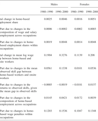
Table 5 presents the results from the statistical decompositions in Equations 4 and 5, separately for males and females, for the 1980–90 and 1990–2000 periods. The upper panel of the table indicates that, for both sexes, the home-based share of wage and salary employment rose by about two-tenths of a percentage point between 1980 and 1990 and by a full half percentage point between 1990 and 2000. Changes over time in the occupational distribution of wage and salary employment can account for 24 (12) percent of the growth in the aggregate male (female) home-based em-ployment share between 1980 and 1990. However, such compositional shifts explain essentially none of the more rapid growth in the aggregate home-based employment shares between 1990 and 2000. Thus, the vast majority of the growth in the home-based share of wage and salary employment in recent decades is explained by in-creases in the frequency of home-based employmentwithinoccupation categories.
Table 5
Decompositions of changes over time in the home-based employment share and the mean log wage gap between home-based and onsite workers, by gender and time period
Males Females
1980–1990 1990–2000 1980–1990 1990–2000
Total change in home-based employment share
0.0025 0.0046 0.0016 0.0051
Part due to changes in the composition of wage and salary employment across occupations
0.0006 ⳮ0.0002 0.0002 0.0003
Part due to changes in home-based employment shares within occupations
0.0019 0.0048 0.0014 0.0048
Total change in mean log wage gap between home-based and onsite workers
0.1904 0.3276 0.1139 0.208
Part due to changes in the mean observed skill gap between home-based workers and onsite workers
0.0561 0.1338 0.0101 0.0536
Part due to changes in the returns to observed skills, given the mean gap in observed skills
ⳮ0.0005 ⳮ0.0019 ⳮ0.0181 0.0157
Part due to changes in the composition of home-based employment across occupations
0.0145 0.0421 0.0172 0.0039
Part due to changes in home-based wage penalties within occupations
0.1203 0.1536 0.1047 0.1348
D. Can IT Explain the Variation in Home-Based Employment Shares and Wage Penalties?
The empirical evidence so far is consistent with the view that broad-based reductions in employer costs of providing home-based jobs have been the main source of growth in the home-based employment share in recent decades. What might have caused these costs to fall? Advances in IT are an obvious possibility. Indeed, recent studies have argued that IT innovations have contributed to the widening of edu-cational wage differentials (Autor, Katz, and Krueger 1998), the rise in female em-ployment and decline in male-female wage differentials (Weinberg 2000), and the adoption of new production methods and organizational practices (Bresnahan, Bryn-jolfsson, and Hitt 2002) in recent decades.
If IT gains were the main reason that employers’ costs of offering home-based jobs fell, one would expect larger increases in home-based employment shares and larger declines in home-based wage penalties to have occurred in gender-occupation categories where these improvements could be utilized more intensively on the typ-ical job. For example, the development and diffusion of technologies allowing elec-tronic file-sharing should have reduced productivity losses and wage penalties from working at home, and therefore should have facilitated growth in home-based work, more for jobs that can readily use these technologies (such as insurance sales agents) than for jobs where these technologies have little application (such as massage ther-apists). In addition, one might expect these effects of IT advances to be larger in jobs where less face-to-face interaction with customers or coworkers is required.
To test these hypotheses, I estimate the regression models in Equation 3. These models seek to explain the variation across gender⳯occupation⳯year cells in
home-based employment shares and home-home-based wage penalties with across-cell variation in (i) the rate of on-the-job IT use and (ii) an interaction between on-the-job IT use and a variable measuring how much face-to-face interaction the job requires — after controlling for gender-occupation fixed effects and year fixed effects. Including gen-der-occupation fixed effects controls for relatively permanent differences in job tasks and production technologies that make some jobs easier to perform from home than others. Including year fixed effects removes any general time trend in home-based employment shares or home-based wage penalties, whatever the source. The esti-mated slope coefficients therefore measure how home-based employment shares and home-based wage penalties have been correlated with on-the-job IT use, and how these effects have been moderated by the extent of required face-to-face interaction on the job, after controlling for common time trends and gender-occupation-specific heterogeneity.
com-munication. Fortuitously, the time between these supplements corresponds reason-ably closely to the ten-year intervals separating the censuses.
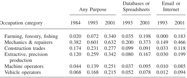
Table 6 displays rates of on-the-job IT use by gender-occupation group and survey year. The first three columns show the fraction of workers in the cell who used a computer on the job for any purpose. On-the-job computer use varied greatly across gender-occupation groups in each year, with much higher usage in professional, managerial, administrative, and sales occupations. Over time, computer use at work has risen dramatically, although the magnitude and timing of this growth has varied across gender-occupation groups. The remaining columns show the fraction of work-ers in the cell who used a computer on the job for database management or spread-sheet programs (Columns 4 and 5) and for email or internet (Columns 6 and 7) in 1993 and 2001. These narrower measures of on-the-job IT use may identify “IT-intensive” gender-occupation categories more accurately, as individuals who used a computer only for inessential activities such as games, music, calendars, or time-keeping are not counted. On-the-job IT use is necessarily lower by these measures, but the general pattern of variation across gender-occupation groups and over time appears similar to the broader measure.
I compute a gender-occupation-specific measure of the importance of in-person interactions on the job using a single cross-section of data from O*NET, the database that succeeded and expanded upon the DOT. O*NET combines survey responses of both job incumbents and professional occupational analysts to describe the required skills, necessary prior training, detailed job tasks, and context of work for over 500 specific occupations.17One element of work context on which data are collected and
that might influence the share of jobs in the occupation that are home-based is how often the work “requires face-to-face discussion with individuals and within teams.” The fraction of responses in five ordinal categories, ranging from “every day” to “never,” is available for each occupation. Using these data, I compute the share of jobs that require less than weekly face-to-face discussion in each of my more ag-gregated gender-occupation groups.18 The percentage of jobs requiring less than
weekly face-to-face discussion ranges from 0.6 percent for male lawyers and judges to 26.5 percent for female retail sales workers. The unweighted mean (standard deviation) across all gender-occupation groups is 11.7 (6.5) percent. In general, professional and managerial occupations are the least likely to require only infre-quent face-to-face interaction.
Because the share of jobs in each gender-occupation group requiring less than weekly face-to-face discussion is measured at only one point in time, the main effect of this variable on home-based employment shares or home-based wage penalties cannot be identified separately from the gender-occupation fixed effect. However,
17. The data used in this study come from O*NET 12.0, which was published in June 2007. The O*NET database first became available in electronic form in 1999, but with more limited data. The DOT never collected the relevant context of work data that is contained in O*NET and also used a different occupa-tional classification system. Consequently, unlike some recent studies such as Autor, Levy, and Murnane (2003), I do not use the DOT data.
Table 6
On-the-job IT use, by gender-occupation category and year
Share of workers who use a computer on the job for:
Any Purpose
Databases or Spreadsheets
Email or Internet
Occupation category 1984 1993 2001 1993 2001 1993 2001
A. Males
Managerial, business 0.452 0.734 0.827 0.444 0.655 0.222 0.721 Engineers, scientists 0.587 0.866 0.918 0.522 0.775 0.368 0.846 Healthcare practitioners 0.358 0.666 0.755 0.283 0.431 0.086 0.542 Teachers, educators 0.367 0.623 0.846 0.236 0.569 0.120 0.733 Arts, media, social service 0.257 0.623 0.785 0.220 0.487 0.121 0.686 Lawyers, judges 0.302 0.667 0.926 0.211 0.549 0.190 0.897 Technicians 0.574 0.734 0.789 0.327 0.538 0.225 0.631 Sales supervisors & reps 0.328 0.639 0.782 0.297 0.549 0.150 0.633 Retail sales 0.184 0.419 0.517 0.111 0.249 0.060 0.266 Office support 0.576 0.801 0.793 0.343 0.546 0.196 0.554 Mail & shipping clerks 0.277 0.555 0.559 0.205 0.330 0.114 0.403 Protective service 0.221 0.457 0.564 0.159 0.299 0.056 0.353 Food or cleaning service 0.037 0.080 0.150 0.019 0.069 0.007 0.082 Health or personal service 0.057 0.154 0.295 0.028 0.140 0.005 0.188 Farming, forestry, fishing 0.015 0.048 0.137 0.008 0.083 0.002 0.096 Mechanics & repairers 0.150 0.310 0.430 0.088 0.208 0.058 0.262 Construction trades 0.040 0.073 0.148 0.026 0.081 0.012 0.090 Extractive, precision
production
0.167 0.361 0.412 0.129 0.221 0.058 0.234
Machine operators 0.097 0.211 0.268 0.055 0.109 0.015 0.123 Vehicle operators 0.035 0.128 0.167 0.014 0.073 0.009 0.074 B. Females
Managerial, business 0.494 0.794 0.862 0.470 0.675 0.254 0.714 Engineers, scientists 0.668 0.838 0.917 0.544 0.719 0.389 0.850 Healthcare practitioners 0.251 0.555 0.740 0.198 0.333 0.065 0.422 Teachers, educators 0.318 0.531 0.766 0.142 0.440 0.062 0.614 Arts, media, social service 0.260 0.600 0.777 0.240 0.425 0.144 0.617 Lawyers, judges 0.277 0.712 0.940 0.128 0.504 0.216 0.865 Technicians 0.430 0.632 0.722 0.273 0.378 0.122 0.447 Sales supervisors & reps 0.416 0.670 0.771 0.296 0.494 0.158 0.573 Retail sales 0.118 0.295 0.389 0.069 0.189 0.019 0.208 Office support 0.498 0.827 0.837 0.353 0.531 0.178 0.563 Mail & shipping clerks 0.510 0.736 0.737 0.306 0.421 0.167 0.489 Protective service 0.202 0.404 0.526 0.147 0.232 0.058 0.296 Food or cleaning service 0.020 0.080 0.159 0.008 0.065 0.004 0.069 Health or personal service 0.056 0.152 0.274 0.033 0.118 0.014 0.132
Table 6(continued)
Share of workers who use a computer on the job for:
Any Purpose
Databases or Spreadsheets
Email or Internet
Occupation category 1984 1993 2001 1993 2001 1993 2001
Farming, forestry, fishing 0.020 0.072 0.340 0.035 0.198 0.000 0.183 Mechanics & repairers 0.382 0.601 0.632 0.200 0.373 0.149 0.466 Construction trades 0.174 0.231 0.277 0.099 0.091 0.033 0.118 Extractive, precision
production
0.120 0.259 0.342 0.080 0.167 0.030 0.199
Machine operators 0.044 0.139 0.251 0.037 0.095 0.010 0.085 Vehicle operators 0.068 0.168 0.215 0.052 0.078 0.012 0.094
Note: Rates of on-the-job IT use are calculated for samples of nonself-employed, civilian workers aged 25–64 from the October 1984, October 1993, and September 2001 Current Population Surveys, using the CPS supplement individual sample weights.
by including an interaction between this variable and the (time-varying) rate of on-the-job IT use in the gender-occupation category in Equation 3, I can investigate whether the effect of on-the-job IT use on based employment shares or home-based wage penalties is moderated by how much face-to-face discussion is required on the job.
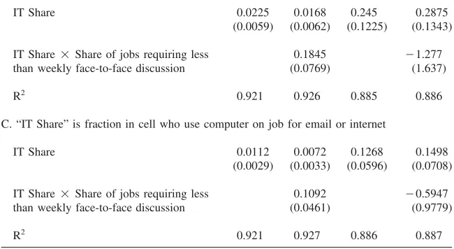
Table 7 reports weighted least squares estimates of Equation 3, where the inverse of the estimated standard error of the dependent variable (the cell-specific home-based employment share or home-home-based wage penalty) is used as the weighting variable. Panel A shows the results when the share of workers in the gen-der⳯occupation⳯year cell who use a computer on the job for any purpose is used as the measure of “IT intensity.” While the point estimates suggest that greater on-the-job IT use is correlated with higher home-based employment shares and smaller (less negative) home-based wage penalties, these relationships are not statistically significant at conventional levels.
Table 7
How on-the-job IT use is related to based employment shares and home-based wage penalties across gender⳯occupation⳯year cells
Dependent variable:
Home-Based Employment Share
Home-Based Wage Penalty
A. “IT Share” is fraction in cell who use computer on job for any purpose
IT Share 0.0107 0.0093 0.0858 0.1449
(0.0060) (0.0061) (0.1205) (0.1246)
IT Share⳯Share of jobs requiring less
than weekly face-to-face discussion
0.0480 ⳮ1.765
(0.0531) (1.086)
R2 0.910 0.911 0.880 0.884
B. “IT Share” is fraction in cell who use computer on job for databases or spreadsheets
IT Share 0.0225 0.0168 0.245 0.2875
(0.0059) (0.0062) (0.1225) (0.1343)
IT Share⳯Share of jobs requiring less
than weekly face-to-face discussion
0.1845 ⳮ1.277
(0.0769) (1.637)
R2 0.921 0.926 0.885 0.886
C. “IT Share” is fraction in cell who use computer on job for email or internet
IT Share 0.0112 0.0072 0.1268 0.1498
(0.0029) (0.0033) (0.0596) (0.0708)
IT Share⳯Share of jobs requiring less
than weekly face-to-face discussion
0.1092 ⳮ0.5947
(0.0461) (0.9779)
R2 0.921 0.927 0.886 0.887
Note: The table reports the estimated slope coefficients and R2values from weighted least squares
The lower panels of Table 7 show that one obtains qualitatively different estimates of Equation 3 using these narrower measures of on-the-job IT use. In Columns 1 and 3, which do not include the interaction term between on-the-job IT use and the share of jobs that require less than weekly face-to-face discussion, the results clearly indicate that home-based employment shares tended to be higher and home-based wage penalties tended to lower (less negative) in cells with higher rates of on-the-job IT use. Again, note that these results hold after controlling for both fixed gender-occupation effects and fixed year effects. Thus, the results indicate that home-based employment shares (wage penalties) grew (shrank) by larger amounts in gender-occupation categories that experienced greater growth in (task-specific measures of) on-the-job IT use.
When the interaction term is added (Columns 2 and 4), its estimated coefficient is positive and significant in the regression explaining home-based employment shares but is negative and insignificant in the regression explaining home-based wage penalties. In both regressions, the main effects of on-the-job IT use on these out-comes are basically unchanged. These results imply that a given increase in on-the-job IT use has tended to be accompanied by a larger increase in the home-based employment share—but not by a larger decline in the home-based wage penalty— in gender-occupation cells where a larger share of jobs require less than weekly face-to-face interaction. Given this mixed result, the main findings from Table 7 are simply that the growth in based employment shares and the decline in home-based wage penalties have been more pronounced in gender-occupation cells with greater growth in on-the-job IT use.
The results in Table 7 are robust to various changes in variable measurement, estimation method, and model specification. For example, the results are qualitatively unchanged when I reestimate the models using a different measure of on-the-job IT use or alternative imputation methods for the 1984 values.19 Likewise, I obtain
comparable results when I reestimate the models by unweighted ordinary least squares. Finally, the results are largely unchanged when I estimate the models with-out year fixed effects, thereby attributing allof the time-series growth (decline) in home-based employment shares (wage penalties) to the growth in on-the-job IT use over time.
In addition, I have checked the robustness of the full set of results reported in the paper in several ways. For example, the results are qualitatively unchanged when I estimate all of the empirical models using samples limited to workers aged 25–55. Likewise, I always obtain essentially identical results to those reported above when I use alternative 1 percent random subsamples of PUMS households with zero home-based workers. Finally, all of the results are virtually unchanged if I use different reasonable rules for imputing topcoded earnings or if I simply drop the topcoded earnings observations from the analyses.
V. Conclusion
This paper has used labor market data from the 1980–2000 U.S. Censuses of Population, supplemented by on-the-job IT use data from the CPS and data on the extent of required face-to-face discussion on the job from O*NET, to analyze how and why the home-based share of employment and the wage penalty on home-based jobs changed between 1980 and 2000. The main findings are: (i) the overall home-based employment share nearly doubled and the mean home-based wage penalty fell by about 30 percentage points over these two decades; (ii) the rise in the home-based employment share and decline in the home-based wage penalty occurred in nearly all major gender-occupation categories and changes in the oc-cupational composition of overall (home-based) employment account for little of the aggregate change in the home-based employment share (wage penalty); and (iii) increases in home-based employment shares and declines in home-based wage pen-alties were larger in gender-occupation cells that saw greater growth in on-the-job IT use for specific work-related tasks.
These findings suggest that falling employer costs of offering home-based work arrangements have been the main factor behind the growth in home-based wage and salary employment over the last several decades and that IT advances were probably an important source of these falling costs. Future research should examine how continued advance and diffusion of IT since 2000 have affected home-based em-ployment shares and home-based wage penalties. Perhaps equally importantly, future research should study how IT gains have influenced other margins of labor supply decisions, including work schedule choices, couples’ colocation decisions, and moth-ers’ employment behavior following childbirth.
References
Abowd, John, and Orley Ashenfelter. 1981. “Anticipated Unemployment, Temporary
Layoffs, and Compensating Wage Differentials.” InStudies in Labor Markets, ed.
Sherwin Rosen, 141–70. Chicago: University of Chicago Press.
Autor, David, Lawrence Katz, and Alan Krueger. 1998. “Computing Inequality: Have
Computers Changed the Labor Market?”Quarterly Journal of Economics113(4): 1169–
213.
Autor, David, Frank Levy, and Richard Murnane. 2003. “The Skill Content of Recent
Technological Change: An Empirical Exploration.”Quarterly Journal of Economics
118(4): 1279–333.
Brown, Charles. 1980. “Equalizing Differences in the Labor Market.”Quarterly Journal of
Economics94(1):113–34.
Bresnahan, Timothy, Erik Brynjolfsson, and Lorin Hitt. 2002. “Information Technology,
Workplace Organization, and the Demand for Skilled Labor.”Quarterly Journal of
Economics117(1):339–76.
Edwards, Linda, and Elizabeth Field-Hendry. 2001. “Work Site and Work Hours: The Labor
Force Flexibility of Home-Based Workers.” InWorking Time in Comparative Perspective,
———. 2002. “Home-Based Work and Women’s Labor Force Decisions.”Journal of Labor Economics20(1):170–200.
Farber, Henry. 1999. “Mobility and Stability: The Dynamics of Job Change in Labor
Markets.” InHandbook of Labor Economics, vol. 3B, ed. Orley Ashenfelter and David
Card, 2439–83. Amsterdam: North-Holland.
Jaeger, David, and Ann Huff Stevens. 1999. “Is Job Stability in the United States Falling? Reconciling Trends in the Current Population Survey and Panel Study of Income
Dynamics.”Journal of Labor Economics17(4): s1–s28.
Kostiuk, Peter. 1990. “Compensating Differentials for Shift Work.”Journal of Political
Economy98(5):1054–75.
Kraut, Robert. 1988. “Homework: What Is It and Who Does It?” InThe New Era of
Home-Based Work: Directions and Policies, ed. Kathleen Christensen, 30–48. Boulder, Colo.: Westview Press.
Kraut, Robert, and Patricia Grambsch. 1987. “Home-Based White Collar Employment:
Lessons from the 1980 Census.”Social Forces66(2):410–26.
Neumark, David, Daniel Polsky, and Daniel Hansen. 1999. “Has Job Stability Declined Yet?
New Evidence for the 1990s.”Journal of Labor Economics17(4): s29–s64.
Olson, Craig. 2002. “Do Workers Accept Lower Wages in Exchange for Health Benefits?”
Journal of Labor Economics20(1): s91–s114.
Pabilonia, Sabrina. 2005. “Working at Home: An Analysis of Telecommuting in Canada.” Unpublished.
Presser, Harriet, and Elizabeth Bamberger. 1993. “American Women who Work at Home for
Pay: Distinctions and Determinants.”Social Science Quarterly74(4):815–37.
Rosen, Sherwin. 1986. “The Theory of Equalizing Differences.” InHandbook of Labor
Economics, vol. 1, ed. Orley Ashenfelter and Richard Layard, 641–92. Amsterdam: North-Holland.
Schroeder, Christine, and Ronald Warren. 2005. “The Effect of Home-Based Work on Earnings.” Unpublished.
Thaler, Richard, and Sherwin Rosen. 1975. “The Value of Saving a Life: Evidence from the
Labor Market.” InHousehold Production and Consumption, ed. N. Terleckyj, 265–302.
New York: Columbia University Press.
Topel, Robert. 1984. “Equilibrium Earnings, Turnover, and Unemployment.”Journal of
Labor Economics2(4):500–22.
Weinberg, Bruce. 2000. “Computer Use and the Demand for Female Workers.”Industrial