http://dx.doi.org/10.12988/ams.2014.47528
A Boussinesq-type Model for Waves
Generated by Flow over a Bump
L.H. Wiryanto
Department of Mathematics, Bandung Institute of Technology Jalan Ganesha 10, Bandung 40132, Indonesia
Sudi Mungkasi
Department of Mathematics, Sanata Dharma University Mrican, Tromol Pos 29, Yogyakarta 55002, Indonesia
Copyright c2014 L. H. Wiryanto and Sudi Mungkasi. This is an open access article distributed under the Creative Commons Attribution License, which permits unrestricted use, distribution, and reproduction in any medium, provided the original work is properly cited.
Abstract
A uniform flow disturbed by a bump is studied. The effect of the disturbance is presented at the surface, generating wave. The wave propagation is modeled into a couple of equations, in terms of the surface elevation and the depth average velocity. The numerical solution of the equations is simulated to observe the propagation, especially for long run time, using a predictor-corrector method. A steady solitary surface profile is obtained for supercritical upstream flow, similarly for subcritical flow but for negative amplitude. In the transient process, more waves are generated but some of them propagates to the left or right, and only one wave remains above the bump.
Mathematics Subject Classification: 35C20, 76B07, 76B25
Keywords: Boussinesq equations, fKdV equation, predictor-corrector method
1
Introduction
described in terms of potential function. Far upstream the flow is uniform with velocity U0 and depth H . The effect of the bump is to generate waves
propagating upstream or downstream from the bump.
We examine the unsteady problem, formulated as Boussinesq-type equa-tions, and solve numerically. Our results indicate that the steady wave is set up when the upstream flow is supercritical, i.e. the Froude numberF =U0/
√
gH
greater than 1. Here g is the acceleration of gravity. The solution is like a solitary wave. This steady wave agrees with one of the solutions obtained by some researchers, such as Forbes and Schwartz [1], Vanden-Broeck [2] and Forbes [3], who solved numerically the steady problem, direct from the exact equations, without approximating the governing equations into a set of equa-tions. Their numerical computations indicated that there were two branches of solutions for F greater than a certain number and greater than 1.
Another approach, the steady problem is approximated into a forced Ko-rteweg de Vries (fKdV) equation. The model contains one non-dimensional parameter Froude number F, and the forcing term representing the bump. Shen et al. [4] derived the fKdV equation, based on Euler equations. Sim-ilarly, for two fluid system, Shen [5] derived the model having a fKdV-type equation, both for interfacial wave and the surface wave. Shen et al. [4] con-firm their results to Forbes and Schwartz [1], two solutions of steady solitary wave. In case the forcing term is a secant-hyperbolic bump, corresponding to the solution of the KdV, Chardar et al. [6] as well as Camassa and Wu [7, 8] ob-tained one solution of secant-hyperbolic-type, only for a certain Froude number depending on the height and width of the bump.
The difference between these two and one solution is then observed by Wiryanto [9]. They derived the model in a form of the fKdV equation, based on the perturbation of the potential function from the uniform flow, and ob-serves the effect of the bump width. The two steady solitary waves tend to a unique solution for a certain number of the width. Less than that number, two solutions with different amplitude are obtained.
2
Boussinesq-type Model
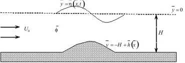
The configuration of the flow over a bump is illustrated in Figure 1. As the system of coordinates, we choose Cartesian with the horizontal ¯x-axis along the undisturbed free surface, and the vertical ¯y-axis perpendicular to the horizontal axis. The bump is described by ¯y = −H + ¯h(¯x). The surface elevation is ¯
y= ¯η(¯x,¯t), with uniform depth H, as ¯x→ −∞, and the potential function is denoted by ¯φ.
The problem is mainly to determine the potential function ¯φ satisfying
¯ for the uniform flow far upstream.
0
Figure 1: Sketch of the flow and coordinates.
Since the potential function tends to uniform flow, written as ¯φ →U0x¯, for
¯
and
The wave, which is generated by the disturbance of the flow, is expressed by the elevation of the surface as ¯y = ¯η(¯x,¯t), with assuming the amplitude
a and wavelength λ. These quantities are then used to scale the variables, together with other quantities, in obtaining the dominant order. To do so, we first define
The next step is to expand the potential function Φ in series of µ2
Φ = Φ0+µ 2
Φ1+µ 4
Φ2+· · ·, (13)
and substituted into (9). It is followed by using the solid boundary (12), so that we have
In this step we separate the variableyfrom the unknown functions Φ0 andφ1,
so that it can help us in applying to the free boundaries (10) and (11).
In expressing (15) and (16) into physical variables, we define the depth average velocity
u= 1
ǫη+ 1−ǫh
Z ǫη
−1+ǫh
Φx(x, y, t)dy.
The approximation ofufor the leading order ofµisu≈Φ0x,so that (15) and
(16) become
ηt+F (ηx+ux−hx) +ǫF (ηxuxx+uxη−uxh) = 0, (17)
ut+F ux+
1
Fηx+ǫF uux = 0. (18)
We obtain (17) by differentiating (16) with respect to x, before replacing Φ0x
byu. Equations (17) and (18) are the model of our problem.
In case ǫ = 0, the linear model can be solved for t → ∞ as the steady solution. The surface elevation is proportional to the bottom topography. The steady linear equations of (17) and (18) can be solved analytically, by eliminating u and then integrating with respect to x. Since the condition
η→0 as |x| → ∞, we obtain
η(x) = F
2
F2
−1h(x). (19) The ratio of the maximum height between the bottom topography and the surface elevation depends on the Froude number of the incoming flow. For supercritical flow F >1, the surface elevation is positive with amplitude de-creasing by inde-creasing F. This can be compared to the solution of the steady fKdV model, having a branch of solution with different amplitude, see for ex-ample in the work of Shen et al. [4] and Wiryanto [9]. Results of (19) indicate that the fKdV solution with high amplitude is unstable. In contrary for sub-critical flow F < 1, the elevation is negative with decreasing amplitude for decreasingF.
3
Numerical Procedure
Now we describe a numerical procedure for solving (17) and (18). The proce-dure is similar to the one used by Wiryanto [10] to solve an interfacial wave model. We write them as
ηt=G(η, ηx, ux, uxx, h, hx), (20)
ut=H(ηx, u, ux), (21)
whereG and H are given by
H=−F ux−
1
Fηx−ǫF uux. (23)
The space domain is discretized uniformly into a finite number of nodes,xi =
i∆x, wherei= 0,1,2, . . . , N −1 for some N. Here ∆x is the space step. The time domain is discretized intotn =n∆t, where n= 0,1,2, . . .. The notation
∆t represents the time step.
We propose to solve the model (17) and (18) using an explicit predictor-corrector method. The predictor step uses the third order Adams-Bashforth formulation
i are the predicted values of η
n+1
i and u
n+1
i ,
respec-tively. These values are then used to compute∗Gn+1
i and∗Hn
+1
i , which are the
predicted values of Gn+1
i and H
n+1
i respectively. The corrector step uses the
third order explicit Adams-Moulton formulation
ηn+1
We use finite difference formulas to discretize equations (22) and (23). Here we use central difference approximation for the space derivativesηx,ux,hx and
uxx. A special treatment is applied for n = 0, i.e. the first iteration of the
method to get η1
i = 0. Note that the initial condition is given by η
0
i = 0 and
u0
i = 0.
4
Numerical Results
Most calculations of the numerical procedure described above use N = 2000 number of nodes, with ∆x = 0.1, ∆t = 0.001 and parameter ǫ = 0.1. The disturbance of the flow is a bump placed at the middle of the domain, presented as a smooth function, such as
h(x) = ssech2
(b(x−xo))−α
The height and width of the bump are presented by s and b. The value
xo is the position of the crest of the bump. The constant α is required to
get zero disturbance at the left and right ends of the interval, h(0) = 0 =
zero, η(x,0) = 0 and u(x,0) = 0. These are followed by analytical boundary conditionsη(0, t) = 0 andu(0, t) = 0, as the left end of the domain is assumed that the flow is uniform.
The numerical calculation is performed by plotting the surface elevation
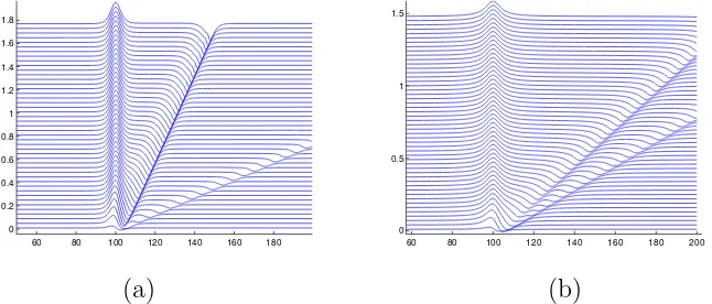
η(x, t). For some different times, the surface elevation is shifted upward, so that we can observe the wave generation and its propagation. Typical plots of surface elevationη for supercritical flow are shown in Figure 2, corresponding to F = 1.5 in Figure 2(a) and F = 4.5 in Figure 2(b). After long run, the negative-amplitude waves have run away from the fluid domain, and solitary-like elevation is as the steady solution, as shown in Figure 2(b). We calculate the plots in Figure 2 using F = 1.5 with s = 0.1, b = 0.3 and α = 0, so the bottom topography is
h(x) = 0.1 sech2
(0.3(x−100)).
With this topography, the values ofh(0) andh(200) are of the orderO(10−27
), which is zero numerically. This means that the condition h(0) = 0 = h(200) is computationally satisfied. The disturbance of the flow causes the surface is lifted up, and increasing the height above the bump, as shown in Figures 2(a) and 2(b), followed by propagating the wave, which is generated on the right side of the bump. The left and right boundaries are set to be absorbing (trans-missive) boundaries by linear extrapolation of η and u. Therefore, the chosen space domain [0,200] is sufficient in the computation. In general, the surface elevation contains one crest and two troughs. As time increases, the surface profile tends to steady with solitary-like. This limiting surface confirms to a solution of the forced KdV model equation, obtained in the work of Shen et al. [4] as well as Wiryanto [9]. In Figure 2, we can compare the wave propa-gation between F = 1.5 and F = 4.5, that the wave speed is larger for larger Froude number. It can be seen the tangential of the wave propagation, the right going waves reach the right boundary faster for larger Froude number.
From the wave evolution in Figure 2(a), we collect the maximum value of
η, namely ηmax for some values t, and we observe that ηmax increases
asymp-totically by increasing the time, higher than the bottom height. We show in Figure 3(a) the plot of ηmax versus time t asymptotically. After t > 25,
ηmax relatively does not change much, i.e. ηmax ≈0.1833. If we compare ηmax
with the bottom height, ηmax is slightly higher than F2/(F2 − 1)hmax, the
maximum value of η for linear steady solution in (19). The value hmax is the
maximum bottom topography of h(x). The surface elevation for that large t
is solitary-like shown in Figure 3(b). Similarly for F = 4.5, for long run we obtain the solitary-like profile, withηmaxsmaller than the result fromF = 1.5,
but approximating toF2
/(F2
−1)hmax.
60 80 100 120 140 160 180 0
0.2 0.4 0.6 0.8 1 1.2 1.4 1.6 1.8
60 80 100 120 140 160 180 200 0
0.5 1 1.5
(a) (b)
Figure 2: Plotη(x, t) for different valuest, (a). Calculated usingF = 1.5, (b).
F = 4.5.
10 20 30 40 50 60
0 0.02 0.04 0.06 0.08 0.1 0.12 0.14 0.16 0.18
Time
Maximum elevation
40 60 80 100 120 140 160 0
0.05 0.1 0.15 0.2
(a) (b)
Figure 3: (a). Plotη(x,160), calculated using F = 1.5, (b). Plotηmax versus
time t.
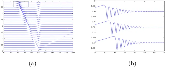
the train of waves is not an error of the calculation.
0 20 40 60 80 100 120 140 160 180 200
0 0.5 1 1.5 2 2.5 3 3.5 4
35 40 45 50 55 60 65 70
3.55 3.6 3.65 3.7 3.75 3.8 3.85 3.9 3.95 4
(a) (b)
Figure 4: (a). Surface elevation η(x, t) for F = 0.6. (b). The zoom of the rectangular-signed inlet in (a).
Similar results, wave generation and its propagation can be observed for other bottom topography, for example a cosine bump in a certain interval and zero in outside that interval. From this unsteady model, a unique solution is obtained. This can be used to identify which stable solution is for the steady model, as there are two solutions for a given bump with supercritical Froude number; see [1, 4, 9].
5
Conclusions
We have derived a Bousinesq-type model for surface wave, generated by flow disturbed by a bump. The unsteady model was solved numerically by a predictor-corrector method, to observe the wave propagation, depending to the incoming flow, presenting by Froude number. As the flow is disturbed by a bump, a wave containing a crest and two troughs is generated. For super-critical flow, both troughs propagate to the right, and the crest is left above the bump, confirms to the result in steady case. Meanwhile, for subcritical the steady case could not be obtained by an fKdV model, as the wave with the crest is going to the left and interacts to the incoming flow.
Australian National University and SMERU Research Institute for the finan-cial support through the Indonesia Project Research Grant 2013/2014.
References
[1] L.K. Forbes and L.W. Schwartz, Free surface flow over a semi-circular obstruction, J. Fluid Mech., 114 (1982), 299–314. http://dx.doi.org/10.1017/S0022112082000160
[2] J.M. Vanden-Broeck, Free surface flow over an obstruction in a channel,
Phys. Fluid, 30 (1987), 2315–2317. http://dx.doi.org/10.1063/1.866121
[3] L.K. Forbes, Critical free-surface flow over a semi-circular obstruction, J.
Eng. Maths., 22 (1988), 3–13. http://dx.doi.org/10.1007/BF00044362
[4] S.P. Shen, M.C. Shen and S. M. Sun, A model equation for steady surface waves over a bump, J. Eng. Maths., 23 (1989), 315–323. http://dx.doi.org/10.1007/BF00128905
[5] S.S.P. Shen, Forced solitary waves and hydraulic falls in two-layer flows, J. Fluid Mech., 234 (1992), 583–612. http://dx.doi.org/10.1017/S0022112092000922
[6] F. Chardar, F. Dias, H.Y. Nguyen and J.M. Vanden-Broeck, Sta-bility of some stationary solutions to the forced KdV equation with one or two bumps, J. Eng. Maths., 70 (2011), 175–189. http://dx.doi.org/10.1007/s10665-010-9424-6
[7] R. Camassa and T.Y. Wu, Stability of forced steady soli-tary waves, Phil. Trans. Royal Soc. A, 337 (1991), 429–466. http://dx.doi.org/10.1098/rsta.1991.0133
[8] R. Camassa and T.Y.T. Wu, Stability of some stationary solutions for the forced KdV equation, Physica D, 51 (1991), 295–307, http://dx.doi.org/10.1016/0167-2789(91)90240-A
[9] L.H. Wiryanto, Numerical solution of a KdV equation, model of a free surface flow, Applied Math. Sci., 8 (2014), 4645–4653. http://dx.doi.org/10.12988/ams.2014.46404
[10] L.H. Wiryanto, Numerical solution of Boussinesq equations as a model of interfacial-wave propagation,Bul. Malay. Math. Sci. Soc., 28 (2005), 163–172.