Statistical Pattern Recognition, 3rd Edition

(1)

PATTERN

RECOGNITION

T h i r d E d i t i o n

Andrew R. Webb

Keith D. Copsey

•

STATISTICAL

(2)

(3)

(4)

(5)

Statistical Pattern Recognition

Third Edition

Andrew R. Webb

_•

Keith D. Copsey

Mathematics and Data Analysis Consultancy, Malvern, UK

(6)

Registered office

John Wiley & Sons Ltd, The Atrium, Southern Gate, Chichester, West Sussex, PO19 8SQ, United Kingdom

For details of our global editorial offices, for customer services and for information about how to apply for permission to reuse the copyright material in this book please see our website at www.wiley.com.

The right of the author to be identified as the author of this work has been asserted in accordance with the Copyright, Designs and Patents Act 1988.

All rights reserved. No part of this publication may be reproduced, stored in a retrieval system, or transmitted, in any form or by any means, electronic, mechanical, photocopying, recording or otherwise, except as permitted by the UK Copyright, Designs and Patents Act 1988, without the prior permission of the publisher.

Wiley also publishes its books in a variety of electronic formats. Some content that appears in print may not be available in electronic books.

Designations used by companies to distinguish their products are often claimed as trademarks. All brand names and product names used in this book are trade names, service marks, trademarks or registered trademarks of their respective owners. The publisher is not associated with any product or vendor mentioned in this book. This publication is designed to provide accurate and authoritative information in regard to the subject matter covered. It is sold on the understanding that the publisher is not engaged in rendering professional services. If professional advice or other expert assistance is required, the services of a competent professional should be sought.

Library of Congress Cataloging-in-Publication Data

Webb, A. R. (Andrew R.)

Statistical pattern recognition / Andrew R. Webb, Keith D. Copsey. – 3rd ed. p. cm.

Includes bibliographical references and index.

ISBN 978-0-470-68227-2 (hardback) – ISBN 978-0-470-68228-9 (paper) 1. Pattern perception–Statistical methods. I. Copsey, Keith D. II. Title.

Q327.W43 2011

006.4–dc23 2011024957

A catalogue record for this book is available from the British Library.

HB ISBN: 978-0-470-68227-2 PB ISBN: 978-0-470-68228-9 ePDF ISBN: 978-1-119-95296-1 oBook ISBN: 978-1-119-95295-4 ePub ISBN: 978-1-119-96140-6 Mobi ISBN: 978-1-119-96141-3

(7)

To Rosemary,

(8)

(9)

Preface

xix

Notation

xxiii

1 Introduction to Statistical Pattern Recognition 1

1.1 Statistical Pattern Recognition 1

1.1.1 Introduction 1

1.1.2 The Basic Model 2

1.2 Stages in a Pattern Recognition Problem 4

1.3 Issues 6

1.4 Approaches to Statistical Pattern Recognition 7

1.5 Elementary Decision Theory 8

1.5.1 Bayes’ Decision Rule for Minimum Error 8

1.5.2 Bayes’ Decision Rule for Minimum Error – Reject Option 12

1.5.3 Bayes’ Decision Rule for Minimum Risk 13

1.5.4 Bayes’ Decision Rule for Minimum Risk – Reject Option 15

1.5.5 Neyman–Pearson Decision Rule 15

1.5.6 Minimax Criterion 18

1.5.7 Discussion 19

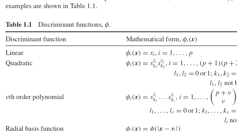
1.6 Discriminant Functions 20

1.6.2 Linear Discriminant Functions 21

1.6.3 Piecewise Linear Discriminant Functions 23

1.6.4 Generalised Linear Discriminant Function 24

1.6.5 Summary 26

1.7 Multiple Regression 27

1.8 Outline of Book 29

1.9 Notes and References 29

Exercises 31

2 Density Estimation – Parametric 33

(10)

2.2 Estimating the Parameters of the Distributions 34

2.2.1 Estimative Approach 34

2.2.2 Predictive Approach 35

2.3 The Gaussian Classifier 35

2.3.1 Specification 35

2.3.2 Derivation of the Gaussian Classifier Plug-In Estimates 37

2.3.3 Example Application Study 39

2.4 Dealing with Singularities in the Gaussian Classifier 40

2.4.2 Na¨ıve Bayes 40

2.4.3 Projection onto a Subspace 41

2.4.4 Linear Discriminant Function 41

2.4.5 Regularised Discriminant Analysis 42

2.4.7 Further Developments 45

2.4.8 Summary 46

2.5 Finite Mixture Models 46

2.5.2 Mixture Models for Discrimination 48

2.5.3 Parameter Estimation for Normal Mixture Models 49

2.5.4 Normal Mixture Model Covariance Matrix Constraints 51

2.5.5 How Many Components? 52

2.5.6 Maximum Likelihood Estimation via EM 55

2.5.9 Summary 63

2.6 Application Studies 63

2.7 Summary and Discussion 66

2.8 Recommendations 66

Exercises 67

3 Density Estimation – Bayesian 70

3.1 Introduction 70

3.1.1 Basics 72

3.1.2 Recursive Calculation 72

3.1.3 Proportionality 73

3.2 Analytic Solutions 73

3.2.1 Conjugate Priors 73

3.2.2 Estimating the Mean of a Normal Distribution with

Known Variance 75

3.2.3 Estimating the Mean and the Covariance Matrix of a Multivariate

Normal Distribution 79

3.2.4 Unknown Prior Class Probabilities 85

3.2.5 Summary 87

3.3 Bayesian Sampling Schemes 87

(11)

CONTENTS ix

3.3.2 Summarisation 87

3.3.3 Sampling Version of the Bayesian Classifier 89

3.3.4 Rejection Sampling 89

3.3.5 Ratio of Uniforms 90

3.3.6 Importance Sampling 92

3.4 Markov Chain Monte Carlo Methods 95

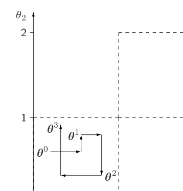
3.4.2 The Gibbs Sampler 95

3.4.3 Metropolis–Hastings Algorithm 103

3.4.4 Data Augmentation 107

3.4.5 Reversible Jump Markov Chain Monte Carlo 108

3.4.6 Slice Sampling 109

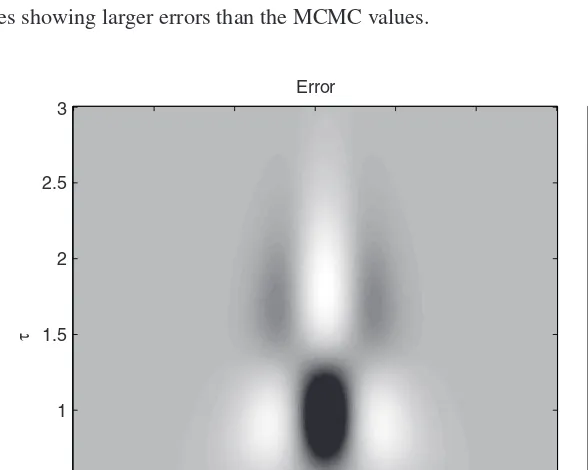
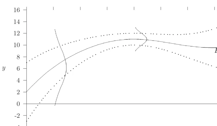
3.4.7 MCMC Example – Estimation of Noisy Sinusoids 111

3.4.8 Summary 115

3.4.9 Notes and References 116

3.5 Bayesian Approaches to Discrimination 116

3.5.1 Labelled Training Data 116

3.5.2 Unlabelled Training Data 117

3.6 Sequential Monte Carlo Samplers 119

3.6.2 Basic Methodology 121

3.6.3 Summary 125

3.7 Variational Bayes 126

3.7.2 Description 126

3.7.3 Factorised Variational Approximation 129

3.7.4 Simple Example 131

3.7.5 Use of the Procedure for Model Selection 135

3.7.6 Further Developments and Applications 136

3.7.7 Summary 137

3.8 Approximate Bayesian Computation 137

3.8.2 ABC Rejection Sampling 138

3.8.3 ABC MCMC Sampling 140

3.8.4 ABC Population Monte Carlo Sampling 141

3.8.5 Model Selection 142

3.8.6 Summary 143

3.9 Example Application Study 144

Exercises 148

4 Density Estimation – Nonparametric 150

4.1 Introduction 150

(12)

4.2 k-Nearest-Neighbour Method 152

4.2.1 k-Nearest-Neighbour Classifier 152

4.2.2 Derivation 154

4.2.3 Choice of Distance Metric 157

4.2.4 Properties of the Nearest-Neighbour Rule 159

4.2.5 Linear Approximating and Eliminating Search Algorithm 159

4.2.6 Branch and Bound Search Algorithms: kd-Trees 163

4.2.7 Branch and Bound Search Algorithms: Ball-Trees 170

4.2.8 Editing Techniques 174

4.2.11 Summary 179

4.3 Histogram Method 180

4.3.1 Data Adaptive Histograms 181

4.3.2 Independence Assumption (Na¨ıve Bayes) 181

4.3.3 Lancaster Models 182

4.3.4 Maximum Weight Dependence Trees 183

4.3.5 Bayesian Networks 186

4.3.6 Example Application Study – Na¨ıve Bayes Text Classification 190

4.3.7 Summary 193

4.4 Kernel Methods 194

4.4.1 Biasedness 197

4.4.2 Multivariate Extension 198

4.4.3 Choice of Smoothing Parameter 199

4.4.4 Choice of Kernel 201

4.4.7 Summary 203

4.5 Expansion by Basis Functions 204

4.6 Copulas 207

4.6.2 Mathematical Basis 207

4.6.3 Copula Functions 208

4.6.4 Estimating Copula Probability Density Functions 209

4.6.5 Simple Example 211

4.6.6 Summary 212

4.7.1 Comparative Studies 216

Exercises 218

5 Linear Discriminant Analysis 221

5.2 Two-Class Algorithms 222

(13)

CONTENTS xi

5.2.2 Perceptron Criterion 223

5.2.3 Fisher’s Criterion 227

5.2.4 Least Mean-Squared-Error Procedures 228

5.2.6 Summary 235

5.3 Multiclass Algorithms 236

5.3.1 General Ideas 236

5.3.2 Error-Correction Procedure 237

5.3.3 Fisher’s Criterion – Linear Discriminant Analysis 238

5.3.4 Least Mean-Squared-Error Procedures 241

5.3.5 Regularisation 246

5.3.8 Summary 248

5.4 Support Vector Machines 249

5.4.2 Linearly Separable Two-Class Data 249

5.4.3 Linearly Nonseparable Two-Class Data 253

5.4.4 Multiclass SVMs 256

5.4.5 SVMs for Regression 257

5.4.6 Implementation 259

5.4.8 Summary 263

5.5 Logistic Discrimination 263

5.5.1 Two-Class Case 263

5.5.2 Maximum Likelihood Estimation 264

5.5.3 Multiclass Logistic Discrimination 266

5.5.6 Summary 268

Exercises 270

6 Nonlinear Discriminant Analysis – Kernel and Projection Methods 274

6.2 Radial Basis Functions 276

6.2.2 Specifying the Model 278

6.2.3 Specifying the Functional Form 278

6.2.4 The Positions of the Centres 279

6.2.5 Smoothing Parameters 281

6.2.6 Calculation of the Weights 282

6.2.7 Model Order Selection 284

(14)

6.2.9 Motivation 286

6.2.10 RBF Properties 288

6.2.13 Summary 290

6.3 Nonlinear Support Vector Machines 291

6.3.2 Binary Classification 291

6.3.3 Types of Kernel 292

6.3.4 Model Selection 293

6.3.5 Multiclass SVMs 294

6.3.6 Probability Estimates 294

6.3.7 Nonlinear Regression 296

6.3.10 Summary 298

6.4 The Multilayer Perceptron 298

6.4.2 Specifying the MLP Structure 299

6.4.3 Determining the MLP Weights 300

6.4.4 Modelling Capacity of the MLP 307

6.4.5 Logistic Classification 307

6.4.7 Bayesian MLP Networks 311

6.4.8 Projection Pursuit 313

6.4.9 Summary 313

Exercises 318

7 Rule and Decision Tree Induction 322

7.2 Decision Trees 323

7.2.2 Decision Tree Construction 326

7.2.3 Selection of the Splitting Rule 327

7.2.4 Terminating the Splitting Procedure 330

7.2.5 Assigning Class Labels to Terminal Nodes 332

7.2.6 Decision Tree Pruning – Worked Example 332

7.2.7 Decision Tree Construction Methods 337

7.2.8 Other Issues 339

(15)

CONTENTS xiii

7.3 Rule Induction 342

7.3.2 Generating Rules from a Decision Tree 345

7.3.3 Rule Induction Using a Sequential Covering Algorithm 345

7.3.6 Summary 351

7.4 Multivariate Adaptive Regression Splines 351

7.4.2 Recursive Partitioning Model 351

7.4.5 Summary 356

Exercises 359

8 Ensemble Methods 361

8.2 Characterising a Classifier Combination Scheme 362

8.2.1 Feature Space 363

8.2.2 Level 366

8.2.3 Degree of Training 368

8.2.4 Form of Component Classifiers 368

8.2.5 Structure 369

8.2.6 Optimisation 369

8.3 Data Fusion 370

8.3.1 Architectures 370

8.3.2 Bayesian Approaches 371

8.3.3 Neyman–Pearson Formulation 373

8.3.4 Trainable Rules 374

8.3.5 Fixed Rules 375

8.4 Classifier Combination Methods 376

8.4.1 Product Rule 376

8.4.2 Sum Rule 377

8.4.3 Min, Max and Median Combiners 378

8.4.4 Majority Vote 379

8.4.5 Borda Count 379

8.4.6 Combiners Trained on Class Predictions 380

8.4.7 Stacked Generalisation 382

8.4.8 Mixture of Experts 382

8.4.9 Bagging 385

8.4.10 Boosting 387

8.4.11 Random Forests 389

(16)

8.4.13 Summary of Methods 396

Exercises 402

9 Performance Assessment 404

9.2 Performance Assessment 405

9.2.1 Performance Measures 405

9.2.2 Discriminability 406

9.2.3 Reliability 413

9.2.4 ROC Curves for Performance Assessment 415

9.2.5 Population and Sensor Drift 419

9.2.8 Summary 423

9.3 Comparing Classifier Performance 424

9.3.1 Which Technique is Best? 424

9.3.2 Statistical Tests 425

9.3.3 Comparing Rules When Misclassification Costs are Uncertain 426

9.3.6 Summary 429

Exercises 431

10 Feature Selection and Extraction 433

10.2 Feature Selection 435

10.2.2 Characterisation of Feature Selection Approaches 439

10.2.3 Evaluation Measures 440

10.2.4 Search Algorithms for Feature Subset Selection 449

10.2.5 Complete Search – Branch and Bound 450

10.2.6 Sequential Search 454

10.2.7 Random Search 458

10.2.8 Markov Blanket 459

10.2.9 Stability of Feature Selection 460

(17)

CONTENTS xv

10.3 Linear Feature Extraction 463

10.3.1 Principal Components Analysis 464

10.3.2 Karhunen–Lo`eve Transformation 475

10.3.5 Summary 483

10.4 Multidimensional Scaling 484

10.4.1 Classical Scaling 484

10.4.2 Metric MDS 486

10.4.3 Ordinal Scaling 487

10.4.4 Algorithms 490

10.4.5 MDS for Feature Extraction 491

10.4.8 Summary 493

Exercises 497

11 Clustering 501

11.2 Hierarchical Methods 502

11.2.1 Single-Link Method 503

11.2.2 Complete-Link Method 506

11.2.3 Sum-of-Squares Method 507

11.2.4 General Agglomerative Algorithm 508

11.2.5 Properties of a Hierarchical Classification 508

11.2.7 Summary 509

11.3 Quick Partitions 510

11.4 Mixture Models 511

11.4.1 Model Description 511

11.5 Sum-of-Squares Methods 513

11.5.1 Clustering Criteria 514

11.5.2 Clustering Algorithms 515

11.5.3 Vector Quantisation 520

11.5.6 Summary 531

11.6 Spectral Clustering 531

11.6.1 Elementary Graph Theory 531

11.6.2 Similarity Matrices 534

11.6.3 Application to Clustering 534

11.6.4 Spectral Clustering Algorithm 535

(18)

11.6.8 Summary 538

11.7 Cluster Validity 538

11.7.2 Statistical Tests 539

11.7.3 Absence of Class Structure 540

11.7.4 Validity of Individual Clusters 541

11.7.5 Hierarchical Clustering 542

11.7.6 Validation of Individual Clusterings 542

11.7.7 Partitions 543

11.7.8 Relative Criteria 543

11.7.9 Choosing the Number of Clusters 545

Exercises 553

12 Complex Networks 555

12.1.1 Characteristics 557

12.1.2 Properties 557

12.1.3 Questions to Address 559

12.1.4 Descriptive Features 560

12.1.5 Outline 560

12.2 Mathematics of Networks 561

12.2.1 Graph Matrices 561

12.2.2 Connectivity 562

12.2.3 Distance Measures 562

12.2.4 Weighted Networks 563

12.2.5 Centrality Measures 563

12.2.6 Random Graphs 564

12.3 Community Detection 565

12.3.1 Clustering Methods 565

12.3.2 Girvan–Newman Algorithm 568

12.3.3 Modularity Approaches 570

12.3.4 Local Modularity 571

12.3.5 Clique Percolation 573

12.3.8 Summary 575

12.4 Link Prediction 575

12.4.1 Approaches to Link Prediction 576

(19)

CONTENTS xvii

Exercises 580

13 Additional Topics 581

13.1 Model Selection 581

13.1.1 Separate Training and Test Sets 582

13.1.2 Cross-Validation 582

13.1.3 The Bayesian Viewpoint 583

13.1.4 Akaike’s Information Criterion 583

13.1.5 Minimum Description Length 584

13.2 Missing Data 585

13.3 Outlier Detection and Robust Procedures 586

13.4 Mixed Continuous and Discrete Variables 587

13.5 Structural Risk Minimisation and the Vapnik–Chervonenkis Dimension 588

13.5.1 Bounds on the Expected Risk 588

13.5.2 The VC Dimension 589

References

591

(20)

(21)

Preface

This book provides an introduction to statistical pattern recognition theory and techniques. Most of the material presented in this book is concerned with discrimination and classification and has been drawn from a wide range of literature including that of engineering, statistics, computer science and the social sciences. The aim of the book is to provide descriptions of many of the most useful of today’s pattern processing techniques including many of the recent advances in nonparametric approaches to discrimination and Bayesian computational methods developed in the statistics literature and elsewhere. Discussions provided on the motivations and theory behind these techniques will enable the practitioner to gain maximum benefit from their implementations within many of the popular software packages. The techniques are illustrated with examples of real-world applications studies. Pointers are also provided to the diverse literature base where further details on applications, comparative studies and theoretical developments may be obtained.

The book grew out of our research on the development of statistical pattern recognition methodology and its application to practical sensor data analysis problems. The book is aimed at advanced undergraduate and graduate courses. Some of the material has been presented as part of a graduate course on pattern recognition and at pattern recognition summer schools. It is also designed for practitioners in the field of pattern recognition as well as researchers in the area. A prerequisite is a knowledge of basic probability theory and linear algebra, together with basic knowledge of mathematical methods (for example, Lagrange multipliers are used to solve problems with equality and inequality constraints in some derivations). Some basic material (which was provided as appendices in the second edition) is available on the book’s website.

Scope

(22)

xx PREFACE

inclusion of some rule induction methods as a complementary approach to rule discovery by decision tree induction.

Most of the methodology is generic – it is not specific to a particular type of data or application. Thus, we exclude preprocessing methods and filtering methods commonly used in signal and image processing.

Approach

The approach in each chapter has been to introduce some of the basic concepts and algorithms and to conclude each section on a technique or a class of techniques with a practical application of the approach from the literature. The main aim has been to introduce the basic concept of an approach. Sometimes this has required some detailed mathematical description and clearly we have had to draw a line on how much depth we discuss a particular topic. Most of the topics have whole books devoted to them and so we have had to be selective in our choice of material. Therefore, the chapters conclude with a section on the key references. The exercises at the ends of the chapters vary from ‘open book’ questions to more lengthy computer projects.

New to the third edition

Many sections have been rewritten and new material added. The new features of this edition include the following:

r

A new chapter on Bayesian approaches to density estimation (Chapter 3) including

expanded material on Bayesian sampling schemes and Markov chain Monte Carlo methods, and new sections on Sequential Monte Carlo samplers and Variational Bayes approaches.

r

New sections on nonparametric methods of density estimation.

r

Rule induction.

r

New chapter on ensemble methods of classification.

r

Revision of feature selection material with new section on stability.

r

Spectral clustering.

r

New chapter on complex networks, with relevance to the high-growth field of social

and computer network analysis.

Book outline

(23)

PREFACE xxi

and a second based on the construction of discriminant functions. The chapter concludes with an outline of the pattern recognition cycle, putting the remaining chapters of the book into context. Chapters 2, 3 and 4 pursue the density function approach to discrimination. Chap-ter 2 addresses parametric approaches to density estimation, which are developed further in Chapter 3 on Bayesian methods. Chapter 4 develops classifiers based on nonparamet-ric schemes, including the popular k nearest neighbour method, with associated efficient search algorithms.

Chapters 5–7 develop discriminant function approaches to supervised classification. Chapter 5 focuses on linear discriminant functions; much of the methodology of this chapter (including optimisation, regularisation, support vector machines) is used in some of the non-linear methods described in Chapter 6 which explores kernel-based methods, in particular, the radial basis function network and the support vector machine, and projection-based meth-ods (the multilayer perceptron). These are commonly referred to as neural network methmeth-ods. Chapter 7 considers approaches to discrimination that enable the classification function to be cast in the form of an interpretable rule, important for some applications.

Chapter 8 considers ensemble methods – combining classifiers for improved robustness. Chapter 9 considers methods of measuring the performance of a classifier.

The techniques of Chapters 10 and 11 may be described as methods of exploratory data analysis or preprocessing (and as such would usually be carried out prior to the supervised classification techniques of Chapters 5–7, although they could, on occasion, be post-processors of supervised techniques). Chapter 10 addresses feature selection and feature extraction – the procedures for obtaining a reduced set of variables characterising the original data. Such procedures are often an integral part of classifier design and it is somewhat artificial to partition the pattern recognition problem into separate processes of feature extraction and classification. However, feature extraction may provide insights into the data structure and the type of classifier to employ; thus, it is of interest in its own right. Chapter 11 considers unsupervised classification orclustering– the process of grouping individuals in a population to discover the presence of structure; its engineering application is to vector quantisation for image and speech coding. Chapter 12 on complex networks introduces methods for analysing data that may be represented using the mathematical concept of a graph. This has great relevance to social and computer networks.

Finally, Chapter 13 addresses some important diverse topics including model selection.

Book website

The websitewww.wiley.com/go/statistical_pattern_recognitioncontains supplementary ma-terial on topics including measures of dissimilarity, estimation, linear algebra, data analysis and basic probability.

Acknowledgements

(24)

xxii PREFACE

who have provided encouragement and made comments on various parts of the manuscript. In particular, we would like to thank Anna Skeoch for providing figures for Chapter 12; and Richard Davies and colleagues at John Wiley for help in the final production of the manuscript. Andrew Webb is especially thankful to Rosemary for her love, support and patience.

(25)

Notation

Some of the more commonly used notation is given below. We have used some notational conveniences. For example, we have tended to use the same symbol for a variable as well as a measurement on that variable. The meaning should be obvious from context. Also, we denote the density function ofxas p(x) andyas p(y), even though the functions differ. A vector is denoted by a lower case quantity in bold face, and a matrix by upper case. Since pattern recognition is very much a multidisciplinary subject, it is impossible to be both consistent across all chapters and consistent with the commonly used notation in the different literatures. We have adopted the policy of maintaining consistency as far as possible within a given chapter.

p,d number of variables

C number of classes

n number of measurements

nj number of measurements in thejth class

ωj label for classj

X1,. . .,Xp prandom variables

x1,. . .,xp measurements on variables,X1,. . .,Xp

x=(x1, . . . ,xp)T measurement vector

X₌[x1, . . . ,xn]T n×pdata matrix

X ₌ ⎡ ⎢ ⎣

x11 . . . x1p

..

. . .. ...

xn1 . . . xnp

⎤ ⎥ ⎦

P(x) = prob(X1≤x1, . . . ,Xp≤xp)

p(x) = ∂P/∂x probability density function

p(x|ωj) probability density function of classj

p(ωj) prior probability of classj

μ = xp(x)dx population mean

μj =

xp(x_|ωj)dx mean of classj,j=1,. . .,C

m₌(1/n) n_i₌₁xi sample mean

mj=(1/nj) n

i=1zjixi sample mean of class j,j = 1,. . ., C; zji =1 if xi∈ωj, 0 otherwise;nj-number of patterns in ωj,nj=

(26)

xxiv NOTATION

ˆ

₌1_n n_i₌₁(xi−m)(xi−m)T sample covariance matrix (maximum likelihood

estimate)

n/(n₋1)ˆ sample covariance matrix (unbiased estimate)

ˆ j= _nj1

n

i=1

zji(xi−mj)(xi−mj)T sample covariance matrix of class j (maximum

likelihood estimate)

Sj = _nnj_j₋1jˆ sample covariance matrix of class j (unbiased

estimate)

SW = Cj=1

nj

nˆj pooled within class sample covariance matrix

S ₌ _nn

−CSW pooled within class sample covariance matrix

(unbiased estimate)

SB= nj_n(mj−m)(mj−m)T sample between class matrix SB+SW = ˆ

A2₌ _ijA2_ij

N(m,) normal (or Gaussian) distribution, mean m,

covariance matrix

N(x_;m,) probability density function for the normal

distribution, mean m, covariance matrix , evaluated atx

E[Y|X] expectation ofYgivenX

(27)

1 Introduction to statistical

pattern recognition

Statistical pattern recognition is a term used to cover all stages of an investigation from problem formulation and data collection through to discrimination and classification, assessment of results and interpretation. Some of the basic concepts in classification are introduced and the key issues described. Two complementary approaches to discrimination are presented, namely a decision theory approach based on calculation of probability density functions and the use of Bayes theorem, and a discriminant function approach.

1.1 Statistical pattern recognition

1.1.1 Introduction

We live in a world where massive amounts of data are collected and recorded on nearly every aspect of human endeavour: for example, banking, purchasing (credit-card usage, point-of-sale data analysis), Internet transactions, performance monitoring (of schools, hospitals, equipment), and communications. The data come in a wide variety of diverse forms – numeric, textual (structured or unstructured), audio and video signals. Understanding and making sense of this vast and diverse collection of data (identifying patterns, trends, anomalies, providing summaries) requires some automated procedure to assist the analyst with this ‘data deluge’. A practical example of pattern recognition that is familiar to many people is classifying email messages (as spam/not spam) based upon message header, content and sender.

Approaches for analysing such data include those for signal processing, filtering, data summarisation, dimension reduction, variable selection, regression and classification and have been developed in several literatures (physics, mathematics, statistics, engineering, artificial intelligence, computer science and the social sciences, among others). The main focus of this book is on pattern recognition procedures, providing a description of basic techniques

(28)

2 INTRODUCTION TO STATISTICAL PATTERN RECOGNITION

together with case studies of practical applications of the techniques on real-world problems. A strong emphasis is placed on the statistical theory of discrimination, but clustering also receives some attention. Thus, the main subject matter of this book can be summed up in a single word: ‘classification’, both supervised (using class information to design a classifier – i.e. discrimination) and unsupervised (allocating to groups without class information – i.e. clustering). However, in recent years many complex datasets have been gathered (for example, ‘transactions’ between individuals – email traffic, purchases). Understanding these datasets requires additional tools in the pattern recognition toolbox. Therefore, we also examine developments such as methods for analysing data that may be represented as a graph.

Pattern recognition as a field of study developed significantly in the 1960s. It was very much an interdisciplinary subject. Some people entered the field with a real problem to solve. The large number of applications ranging from the classical ones such as automatic character recognition and medical diagnosis to the more recent ones indata mining(such as credit scor-ing, consumer sales analysis and credit card transaction analysis) have attracted considerable research effort with many methods developed and advances made. Other researchers were motivated by the development of machines with ‘brain-like’ performance, that in some way could operate giving human performance.

Within these areas significant progress has been made, particularly where the domain over-laps with probability and statistics, and in recent years there have been many exciting new developments, both in methodology and applications. These build on the solid foundations of earlier research and take advantage of increased computational resources readily avail-able nowadays. These developments include, for example, kernel-based methods (including support vector machines) and Bayesian computational methods.

The topics in this book could easily have been described under the termmachine learning

that describes the study of machines that can adapt to their environment and learn from exam-ple. The machine learning emphasis is perhaps more on computationally intensive methods and less on a statistical approach, but there is strong overlap between the research areas of statistical pattern recognition and machine learning.

1.1.2 The basic model

Since many of the techniques we shall describe have been developed over a range of diverse disciplines, there is naturally a variety of sometimes contradictory terminology. We shall use the term ‘pattern’ to denote thep-dimensional data vectorx₌(x1, . . . ,xp)Tof measurements

(T _{denotes vector transpose), whose components}_xi_{are measurements of the features of an}

object. Thus the features are the variables specified by the investigator and thought to be important for classification. In discrimination, we assume that there existCgroups orclasses, denotedω1,. . .,ωCand associated with each patternxis a categorical variablezthat denotes

the class or group membership; that is, ifz=i, then the pattern belongs toωi,i∈{1,. . .,C}.

(29)

STATISTICAL PATTERN RECOGNITION 3

Figure 1.1 Pattern classifier.

The main topic in this book may be described by a number of terms including pattern classifier design or discrimination or allocation rule design. Designing the rule requires specification of the parameters of a pattern classifier, represented schematically in Figure 1.1, so that it yields the optimal (in some sense) response for a given input pattern. This response is usually an estimate of the class to which the pattern belongs. We assume that we have a set of patterns of known class_{(xi,zi),i=1, . . . ,n}(thetrainingordesignset) that we use

to design the classifier (to set up its internal parameters). Once this has been done, we may estimate class membership for a patternxfor which the class label is unknown. Learning the model from a training set is the process ofinduction; applying the trained model to patterns of unknown class is the process ofdeduction.

Thus, the uses of a pattern classifier are to provide:

r

A descriptive model that explains the difference between patterns of different classes

in terms of features and their measurements.

r

A predictive model that predicts the class of an unlabelled pattern.

However, we might ask why do we need a predictive model? Cannot the procedure that was used to assign labels to the training set measurements also be used for the test set in classifier operation? There may be several reasons for developing an automated process:

r

to remove humans from the recognition process – to make the process more reliable;

r

in banking, to identify good risk applicants before making a loan;

r

to make a medical diagnosis without a post mortem (or to assess the state of a piece of

equipment without dismantling it) – sometimes a pattern may only be labelled through intensive examination of a subject, whether person or piece of equipment;

r

to reduce cost and improve speed – gathering and labelling data can be a costly and

time consuming process;

r

to operate in hostile environments – the operating conditions may be dangerous or

harmful to humans and the training data have been gathered under controlled conditions;

r

to operate remotely – to classify crops and land use remotely without labour-intensive,

time consuming, surveys.

(30)

made concerning its distribution. Another important factor is the misclassification cost – the cost of making an incorrect decision. In many applications misclassification costs are hard to quantify, being combinations of several contributions such as monetary costs, time and other more subjective costs. For example, in a medical diagnosis problem, each treatment has different costs associated with it. These relate to the expense of different types of drugs, the suffering the patient is subjected to by each course of action and the risk of further complications.

Figure 1.1 grossly oversimplifies the pattern classification procedure. Data may undergo several separate transformation stages before a final outcome is reached. These transforma-tions (sometimes termed preprocessing, feature selection or feature extraction) operate on the data in a way that, usually, reduces its dimension (reduces the number of features), removing redundant or irrelevant information, and transforms it to a form more appropriate for sub-sequent classification. The termintrinsic dimensionalityrefers to the minimum number of variables required to capture the structure within the data. In speech recognition, a prepro-cessing stage may be to transform the waveform to a frequency representation. This may be processed further to find formants (peaks in the spectrum). This is afeature extractionprocess (taking a possibly nonlinear combination of the original variables to form new variables). Fea-ture selectionis the process of selecting a subset of a given set of variables (see Chapter 10). In some problems, there is no automatic feature selection stage, with the feature selection being performed by the investigator who ‘knows’ (through experience, knowledge of previous studies and the problem domain) those variables that are important for classification. In many cases, however, it will be necessary to perform one or more transformations of the measured data.

In some pattern classifiers, each of the above stages may be present and identifiable as separate operations, while in others they may not be. Also, in some classifiers, the preliminary stages will tend to be problem specific, as in the speech example. In this book, we consider feature selection and extraction transformations that are not application specific. That is not to say the methods of feature transformation described will be suitable for any given application, however, but application-specific preprocessing must be left to the investigator who understands the application domain and method of data collection.

1.2 Stages in a pattern recognition problem

A pattern recognition investigation may consist of several stages enumerated below. Not all stages may be present; some may be merged together so that the distinction between two operations may not be clear, even if both are carried out; there may be some application-specific data processing that may not be regarded as one of the stages listed below. However, the points below are fairly typical.

1. Formulation of the problem: gaining a clear understanding of the aims of the investi-gation and planning the remaining stages.

(31)

STAGES IN A PATTERN RECOGNITION PROBLEM 5

3. Initial examination of the data: checking the data, calculating summary statistics and producing plots in order to get a feel for the structure.

4. Feature selection or feature extraction: selecting variables from the measured set that are appropriate for the task. These new variables may be obtained by a linear or nonlinear transformation of the original set (feature extraction). To some extent, the partitioning of the data processing into separate feature extraction and classification processes is artificial, since a classifier often includes the optimisation of a feature extraction stage as part of its design.

5. Unsupervised pattern classification or clustering. This may be viewed as exploratory data analysis and it may provide a successful conclusion to a study. On the other hand, it may be a means of preprocessing the data for a supervised classification procedure.

6. Apply discrimination or regression procedures as appropriate. The classifier is designed using a training set of exemplar patterns.

7. Assessment of results. This may involve applying the trained classifier to an indepen-denttest setof labelled patterns. Classification performance is often summarised in the form of a confusion matrix:

True class

ω1 ω2 ω3

Predicted class ω1 e11 e12 e13

ω2 e21 e22 e23

ω3 e31 e32 e33

whereeijis the number of patterns of classωjthat are predicted to be classωi. The

accuracy,a, is calculated from the confusion matrix as

a₌

i eii

ij eij

and the error rate is 1₋a.

8. Interpretation.

The above is necessarily an iterative process: the analysis of the results may generate new hypotheses that require further data collection. The cycle may be terminated at different stages: the questions posed may be answered by an initial examination of the data or it may be discovered that the data cannot answer the initial question and the problem must be reformulated.

(32)

1.3 Issues

The main topic that we address in this book concerns classifier design: given a training set of patterns of known class, we seek to use those examples to design a classifier that is optimal for the expected operating conditions (the test conditions).

There are a number of very important points to make about this design process.

Finite design set

We are given a finite design set. If the classifier is too complex (there are too many free parameters) it may model noise in the design set. This is an example ofoverfitting. If the classifier is not complex enough, then it may fail to capture structure in the data. An illustration of this is the fitting of a set of data points by a polynomial curve (Figure 1.2). If the degree of the polynomial is too high then, although the curve may pass through or close to the data points thus achieving a low fitting error, the fitting curve is very variable and models every fluctuation in the data (due to noise). If the degree of the polynomial is too low, the fitting error is large and the underlying variability of the curve is not modelled (the modelunderfitsthe data). Thus, achieving optimal performance on the design set (in terms of minimising some error criterion perhaps) is not required: it may be possible, in a classification problem, to achieve 100% classification accuracy on the design set but thegeneralisation performance– the expected performance on data representative of the true operating conditions (equivalently the performance on an infinite test set of which the design set is a sample) – is poorer than could be achieved by careful design. Choosing the ‘right’ model is an exercise inmodel selection. In practice we usually do not know what is structure and what is noise in the data. Also, training a classifier (the procedure of determining its parameters) should not be considered as a separate issue from model selection, but it often is.

–0.4 –0.2 0.2 0.4

–0.1 0.1 0.2

(33)

APPROACHES TO STATISTICAL PATTERN RECOGNITION 7

Optimality

A second point about the design of optimal classifiers concerns the word ‘optimal’. There are several ways of measuring classifier performance, the most common being error rate, although this has severe limitations (see Chapter 9). Other measures, based on the closeness of the estimates of the probabilities of class membership to the true probabilities, may be more appropriate in many cases. However, many classifier design methods usually optimise alternative criteria since the desired ones are difficult to optimise directly. For example, a classifier may be trained by optimising a square-error measure and assessed using error rate.

Representative data

Finally, we assume that the training data are representative of the test conditions. If this is not so, perhaps because the test conditions may be subject to noise not present in the training data, or there are changes in the population from which the data are drawn (population drift), then these differences must be taken into account in the classifier design.

1.4 Approaches to statistical pattern recognition

There are two main divisions of classification:supervised classification(or discrimination) andunsupervised classification(sometimes in the statistics literature simply referred to as classification or clustering).

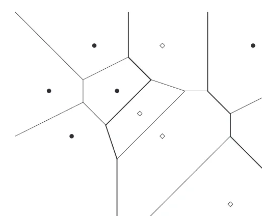
The problem we are addressing in this book is primarily one ofsupervised pattern clas-sification. Given a set of measurements obtained through observation and represented as a pattern vectorx, we wish to assign the pattern to one ofCpossible classes,ωi,i=1,. . ., C. Adecision rulepartitions the measurement space intoCregions,i,i=1,. . .,C. If an

observation vector is inithen it is assumed to belong to classωi. Each class regionimay

be multiply connected – that is, it may be made up of several disjoint regions. The boundaries between the regionsi are thedecision boundariesordecision surfaces. Generally, it is in

regions close to these boundaries where the highest proportion of misclassifications occurs. In such situations, we may reject the pattern or withhold a decision until further information is available so that a classification may be made later. This option is known as thereject option

and therefore we haveC₊1 outcomes of a decision rule (the reject option being denoted by

ω0) in aCclass problem:xbelongs toω1orω2or. . . orωCor withhold a decision.

In unsupervised classification, the data are not labelled and we seek to find groups in the data and the features that distinguish one group from another. Clustering techniques, described further in Chapter 11, can also be used as part of a supervised classification scheme by defining prototypes. A clustering scheme may be applied to the data for each class separately and representative samples for each group within the class (the group means for example) used as the prototypes for that class.

In the following section we introduce two approaches to discrimination that will be explored further in later chapters. The first assumes a knowledge of the underlying class-conditional probability density functions (the probability density function of the feature vectors for a given class). Of course, in many applications these will usually be unknown and must be estimated from a set of correctly classified samples termed thedesignor training

set. Chapters 2, 3 and 4 describe techniques for estimating the probability density functions explicitly.

(34)

density functions. This approach is developed in Chapters 5 and 6 where specific techniques are described.

1.5 Elementary decision theory

Here we introduce an approach to discrimination based on knowledge of the probability density functions of each class. Familiarity with basic probability theory is assumed.

1.5.1 Bayes’ decision rule for minimum error

ConsiderC classes,ω1,. . .,ωC, witha priori probabilities (the probabilities of each class

occurring) p(ω1),. . ., p(ωC), assumed known. If we wish to minimise the probability of

making an error and we have no information regarding an object other than the class probability distribution then we would assign an object to classωjif

p(ωj) >p(ωk) k=1, . . . ,C;k= j

This classifies all objects as belonging to one class: the class with the largest prior prob-ability. For classes with equal prior probabilities, patterns are assigned arbitrarily between those classes.

However, we do have anobservation vector or measurement vectorx and we wish to assign an object to one of theCclasses based on the measurementsx. A decision rule based on probabilities is to assignx(here we refer to an object in terms of its measurement vector) to classωj if the probability of classωj given the observationx, that is p(ωj|x), is greatest

over all classesω1,. . .,ωC. That is, assignxto classωjif

p(ωj|x) >p(ωk|x) k=1, . . . ,C;k= j (1.1)

This decision rule partitions the measurement space intoCregions1,. . .,Csuch that if

x_∈jthenxbelongs to classωj. The regionsjmay be disconnected.

Thea posterioriprobabilitiesp(ωj_|x)may be expressed in terms of thea priori probabil-ities and the class conditional density functionsp(x_|ωi)using Bayes’ theorem as

p(ωi|x)=

p(x_|ωi)p(ωi) p(x)

and so the decision rule (1.1) may be written: assignxtoωjif

p(x_|ωj)p(ωj) >p(x|ωk)p(ωk) k=1, . . . ,C;k= j (1.2)

This is known as Bayes’ rule forminimum error.

For two classes, the decision rule (1.2) may be written

lr(x)=

p(x_|ω1)

p(x_|ω2)

> p(ω2) p(ω1)

(35)

ELEMENTARY DECISION THEORY 9

A

0 0.02 0.04 0.06 0.08 0.1 0.12 0.14 0.16 0.18 0.2

-4 -3 -2 -1 0 1 2 3 4

x

p(x|ω2)p(ω2) p(x|ω1)p(ω1)

Figure 1.3 p(x_|ωi)p(ωi), for classesω1andω2: forxin regionA,xis assigned to classω1.

The functionlr(x)is thelikelihood ratio. Figures 1.3 and 1.4 give a simple illustration for a

two-class discrimination problem. Classω1 is normally distributed with zero mean and unit

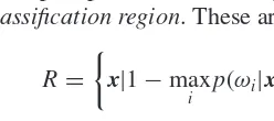
variance,p(x_|ω1)=N(x;0,1). Classω2is anormal mixture(a weighted sum of normal

den-sities) p(x_|ω2)=0.6N(x;1,1)+0.4N(x; −1,2). Figure 1.3 plots p(x|ωi)p(ωi),i=1,2,

where the priors are taken to bep(ω1)=0.5,p(ω2)=0.5. Figure 1.4 plots the likelihood ratio

lr(x)and the thresholdp(ω2)/p(ω1). We see from this figure that the decision rule (1.2) leads

to a disconnected region for classω2.

x A

0 0.2 0.4 0.6 0.8 1 1.2 1.4 1.6 1.8 2

-4 -3 -2 -1 0 1 2 3 4

lr(x)

p(ω2)/p(ω1)

(36)

The fact that the decision rule (1.2) minimises the error may be seen as follows. The probability of making an error,p(error), may be expressed as

p(error)₌ C

i=1

p(error_|ωi)p(ωi) (1.3)

wherep(error_|ωi) is the probability of misclassifying patterns from classωi. This is given by

p(error_|ωi)=

C[i]

p(x_|ωi)dx (1.4)

the integral of the class-conditional density function overC[i], the region of measurement

space outsidei(Cis the complement operator), i.e.

C

j=1,j=ij. Therefore, we may write

the probability of misclassifying a pattern as

p(error)₌

from which we see that minimising the probability of making an error is equivalent to maximising

which is the probability of correct classification. Therefore, we wish to choose the regions

iso that the integral given in (1.6) is a maximum. This is achieved by selecting i to be

the region for whichp(ωi)p(x|ωi)is the largest over all classes and the probability of correct

classification,c, is

c₌

max

i p(ωi)p(x|ωi)dx (1.7)

where the integral is over the whole of the measurement space, and the Bayes’ error is

eB=1−

max

i p(ωi)p(x|ωi)dx (1.8)

(37)

xB

0 0.05 0.1 0.15 0.2

0.25 0.3 0.35 0.4

-4 -3 -2 -1 0 1 2 3 4

p(x|ω2)

p(x|ω1)

Figure 1.5 Class-conditional densities for two normal distributions.

Figure 1.5 plots the two distributions p(x|ωi),i=1,2 (both normal with unit variance

and means±0.5), and Figure 1.6 plots the functionsp(x|ωi)p(ωi)wherep(ω1)=0.3,p(ω2)=

0.7. The Bayes’ decision boundary defined by the point wherep(x_|ω1)p(ω1)=p(x|ω2)p(ω2)

(Figure 1.6) is marked with a vertical line atxB. The areas of the hatched regions in Figure 1.5

represent the probability of error: by Equation (1.4), the area of the horizontal hatching is the probability of classifying a pattern from class 1 as a pattern from class 2 and the area of the vertical hatching the probability of classifying a pattern from class 2 as class 1. The sum of these two areas, weighted by the priors [Equation (1.5)], is the probability of making an error.

xB

0 0.05 0.1 0.15 0.2

0.25 0.3

-4 -3 -2 -1 0 1 2 3 4

p(x|ω2)p(ω2)

p(x|ω1)p(ω1)

(38)

1.5.2 Bayes’ decision rule for minimum error – reject option

As we have stated above, an error or misrecognition occurs when the classifier assigns a pattern to one class when it actually belongs to another. In this section we consider the reject option. Usually it is the uncertain classifications (often close to the decision boundaries) that contribute mainly to the error rate. Therefore, rejecting a pattern (withholding a decision) may lead to a reduction in the error rate. This rejected pattern may be discarded, or set aside until further information allows a decision to be made. Although the option to reject may alleviate or remove the problem of a high misrecognition rate, some otherwise correct classifications are also converted into rejects. Here we consider the trade-offs between error rate and reject rate. First, we partition the sample space into two complementary regions:R, areject region

andA, anacceptanceorclassification region. These are defined by

R₌

x_|1₋max

i p(ωi|x) >t

A=

x_|1−max

i p(ωi|x)≤t

wheretis a threshold. This is illustrated in Figure 1.7 using the same distributions as those in Figures 1.5 and 1.6.

The smaller the value of the thresholdtthen the larger is the reject regionR. However, if

tis chosen such that

1−t ≤ 1

C

or equivalently,

t≥C−1

C

1−t t

A R A

0 0.1 0.2

0.3 0.4

0.5 0.6 0.7 0.8

0.9 1

-4 -3 -2 -1 0 1 2 3 4

p(ω1|x)

p(ω2|x)

(39)

whereCis the number of classes, then the reject region is empty. This is because the minimum value which max

i p(ωi|x)can attain is 1/C[since 1=

C

i=1p(ωi|x)≤Cmax

i p(ωi|x)], when

all classes are equally likely. Therefore, for the reject option to be activated, we must have

t<(C−1)/C.

Thus, if a patternxlies in the regionA, we classify it according to the Bayes’ rule for minimum error [Equation (1.2)]. However, ifxlies in the regionR, we rejectx(withhold a decision).

The probability of correct classification,c(t), is a function of the threshold,t, and is given by Equation (1.7), where now the integral is over the acceptance region,A, only

c(t)₌

A

max

i [p(ωi)p(x|ωi)]dx

and the unconditional probability of rejecting a measurement,r, also a function of the threshold

t, is the probability that it lies inR:

r(t)₌

R

p(x)dx (1.9)

Therefore, the error rate,e(the probability of accepting a point for classification and incorrectly classifying it), is

Thus, the error rate and reject rate are inversely related. Chow (1970) derives a simple functional relationship betweene(t) andr(t) which we quote here without proof. Knowing

r(t) over the complete range oftallowse(t) to be calculated using the relationship

e(t)_{= −}

t

0

sdr(s) (1.10)

The above result allows the error rate to be evaluated from the reject function for the Bayes’ optimum classifier. The reject function can be calculated usingunlabelleddata and a practical application of the above result is to problems where labelling of gathered data is costly.

1.5.3 Bayes’ decision rule for minimum risk

In the previous section, the decision rule selected the class for which thea posteriori prob-ability, p(ωj|x), was the greatest. This minimised the probability of making an error. We

(40)

We make this concept more formal by introducing a loss that is a measure of the cost of making the decision that a pattern belongs to classωiwhen the true class isωj. We define a

loss matrixwith components

λji=cost of assigning a patternxtoωiwhenx∈ωj

In practice, it may be very difficult to assign costs. In some situations,λmay be measured in monetary units that are quantifiable. However, in many situations, costs are a combination of several different factors measured in different units – money, time, quality of life. As a consequence, they are often a subjective opinion of an expert. Theconditional riskof assigning a patternxto classωiis defined as

The average risk over regioniis

ri₌

and the overall expected cost orriskis

r=

The above expression for the risk will be minimised if the regionsiare chosen such that if

C

One special case of the loss matrixis theequal costloss matrix for which

λij=

1 i= j

(41)

Substituting into (1.12) gives the decision rule: assignxto classωiif C

implies thatx_∈classωi; this is the Bayes’ rule for minimum error.

1.5.4 Bayes’ decision rule for minimum risk – reject option

As with the Bayes’ rule for minimum error, we may also introduce a reject option, by which the reject region,R, is defined by

R=

wheretis a threshold. The decision is to accept a patternxand assign it to classωiif

li(x)₌min

This decision is equivalent to defining a reject region0with a constant conditional risk

l0(x)₌t

so that the Bayes’ decision rule is: assignxto classωiif

li(x)_≤lj(x) j=0,1, . . . ,C

(42)

decision process. We may classify a pattern of classω1as belonging to classω2 or a pattern

from classω2as belonging to classω1. Let the probability of these two errors beǫ1andǫ2,

The Neyman–Pearson decision rule is to minimise the errorǫ1subject toǫ2being equal to a

constant,ǫ0, say.

If classω1 is termed the positive class and class ω2 the negative class, thenǫ1 is

re-ferred to as thefalse negative rate: the proportion of positive samples incorrectly assigned to the negative class;ǫ2is thefalse positive rate: the proportion of negative samples classed

as positive.

An example of the use of the Neyman–Pearson decision rule is in radar detection where the problem is to detect a signal in the presence of noise. There are two types of error that may occur; one is to mistake noise for a signal present. This is called afalse alarm. The second type of error occurs when a signal is actually present but the decision is made that only noise is present. This is amissed detection. Ifω1denotes the signal class andω2denotes the noise

thenǫ2is the probability of false alarm andǫ1is the probability of missed detection. In many

radar applications, a threshold is set to give a fixed probability of false alarm and therefore the Neyman–Pearson decision rule is the one usually used.

We seek the minimum of

r₌

whereμis a Lagrange multiplier1_and_ǫ

0is the specified false alarm rate. The equation may

be written

r₌(1₋μǫ0)+

1

{μp(x_|ω2)dx−p(x|ω1)dx}

This will be minimised if we choose1such that the integrand is negative, i.e.

ifμp(x|ω2)−p(x|ω1) <0,thenx∈1

or, in terms of the likelihood ratio,

if p(x|ω1)

p(x_|ω2)

> μ,thenx_∈1 (1.14)

1_{The method of Lagrange’s undetermined multipliers can be found in most textbooks on mathematical methods,}

(43)

Thus the decision rule depends only on the within-class distributions and ignores thea priori

probabilities.

The thresholdμis chosen so that

1

p(x_|ω2)dx=ǫ0,

the specified false alarm rate. However, in generalμcannot be determined analytically and requires numerical calculation.

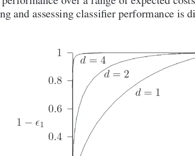
Often, the performance of the decision rule is summarised in a receiver operating char-acteristic (ROC) curve, which plots the true positive against the false positive (that is, the probability of detection [1−ǫ1=

1p(x|ω1)dx] against the probability of false alarm

[ǫ2=

1p(x|ω2)dx)] as the thresholdμis varied. This is illustrated in Figure 1.8 for the

univariate case of two normally distributed classes of unit variance and means separated by a distance,d. All the ROC curves pass through the (0, 0) and (1, 1) points and as the separation increases the curve moves into the top left corner. Ideally, we would like 100% detection for a 0% false alarm rate and curves that are closer to this the better.

For the two-class case, the minimum risk decision [see Equation (1.12)] defines the decision rules on the basis of the likelihood ratio (λii=0):

if p(x|ω1)

p(x_|ω2)

> λ21p(ω2) λ12p(ω1)

,thenx_∈1 (1.15)

The threshold defined by the right-hand side will correspond to a particular point on the ROC curve that depends on the misclassification costs and the prior probabilities.

In practice, precise values for the misclassification costs will be unavailable and we shall need to assess the performance over a range of expected costs. The use of the ROC curve as a tool for comparing and assessing classifier performance is discussed in Chapter 9.

0 0.2

0.4

0.6 0.8

1

0 0.2 0.4 0.6 0.8 1

1−ǫ1

ǫ2 d= 1

d=2 d=4

Figure 1.8 Receiver operating characteristic for two univariate normal distributions of unit variance and separation,d; 1−ǫ1=₁p(x|ω1)dx is the true positive (the probability of

detection) andǫ2=

(44)

1.5.6 Minimax criterion

The Bayes’ decision rules rely on a knowledge of both the within-class distributions and the prior class probabilities. However, situations may arise where the relative frequencies of new objects to be classified are unknown. In this situation aminimaxprocedure may be employed. The nameminimaxis used to refer to procedures for which either the maximum expected loss

orthe maximum of the error probability is a minimum. We shall limit our discussion below to the two-class problem and the minimum error probability procedure.

Consider the Bayes’ rule for minimum error. The decision regions1and2are defined by

p(x_|ω1)p(ω1) >p(x|ω2)p(ω2)impliesx∈1 (1.16)

and the Bayes’ minimum error,eB, is

eB=p(ω2)

1

p(x|ω2)dx+p(ω1)

2

p(x|ω1)dx (1.17)

wherep(ω2)=1−p(ω1).

Forfixed decision regions1 and2,eB is a linear function ofp(ω1) (we denote this

functione_˜B) attaining its maximum on the region [0, 1] either atp(ω1)=0 orp(ω1)=1.

However, since the regions 1 and 2 are also dependent on p(ω1) through the Bayes’

decision criterion (1.16), the dependency ofeBonp(ω1) is more complex, and not necessarily

monotonic.

If1and2are fixed [determined according to (1.16) for some specifiedp(ωi)], the error

given by (1.17) will only be the Bayes’ minimum error for a particular value ofp(ω1), sayp∗1

(Figure 1.9).

For other values ofp(ω1), the error given by (1.17) must be greater than the minimum

error. Therefore, the optimum curve touches the line at a tangent at p∗₁and is concave down at that point.

0 .

0 1.0

a b

Bayes’ minimum error,eB

error, ˜eB, for fixed

decision regions

p∗

1 p(ω1)

(45)

The minimax procedure aims to choose the partition1,2, or equivalently the value of

p(ω1) so that the maximum error (on a test set in which the values ofp(ωi) are unknown)

is minimised. For example, in Figure 1.9, if the partition were chosen to correspond to the valuep∗₁ofp(ω1), then the maximum error which could occur would be a value ofbifp(ω1)

were actually equal to unity. The minimax procedure aims to minimise this maximum value, i.e. minimise

This is a minimum when

minimum error curve at its peak value.

Therefore, we choose the regions1and2so that the probabilities of the two types of

error are the same. The minimax solution may be criticised as being over-pessimistic since it is a Bayes’ solution with respect to the least favourable prior distribution. The strategy may also be applied to minimising the maximum risk. In this case, the risk is

and the boundary must therefore satisfy

λ11−λ22+(λ12−λ11)

Statistical Pattern Recognition, 3rd Edition

PATTERN

RECOGNITION

T h i r d E d i t i o n

Andrew R. Webb

Keith D. Copsey

•

•

•

•

•

•

•

STATISTICAL

Statistical Pattern Recognition

Third Edition

Andrew R. Webb

•

Keith D. Copsey

Mathematics and Data Analysis Consultancy, Malvern, UK

To Rosemary,

Contents

Preface

xix

Notation

xxiii

References

591

Preface

Scope

Approach

New to the third edition

r

r

r

r

r

r

r

Book outline

Book website

Acknowledgements

Notation

1

Introduction to statistical

pattern recognition

1.1

Statistical pattern recognition

1.1.1

Introduction

1.1.2

The basic model

r

r

r

r

r

r

r

r

1.2

Stages in a pattern recognition problem

1.3

Issues

1.4

Approaches to statistical pattern recognition

1.5

Elementary decision theory

1.5.1

Bayes’ decision rule for minimum error

1.5.2

Bayes’ decision rule for minimum error – reject option

1.5.3

Bayes’ decision rule for minimum risk

1.5.4

Bayes’ decision rule for minimum risk – reject option

1.5.6

Minimax criterion

_•