Contents lists available atScienceDirect
Operations Research Perspectives
journal homepage:www.elsevier.com/locate/orp
Pricing decision model for new and remanufactured short-life cycle products
with time-dependent demand
Shu San Gan
a,c, I. Nyoman Pujawan
a,∗, Suparno
a, Basuki Widodo
baDepartment of Industrial Engineering - Faculty of Industrial Technology, Sepuluh Nopember Institute of Technology, Surabaya 60111, Indonesia bDepartment of Mathematics - Faculty of Mathematics and Natural Science Sepuluh Nopember Institute of Technology, Surabaya 60111, Indonesia cDepartment of Mechanical Engineering - Faculty of Industrial Technology, Petra Christian University, Surabaya 60236, Indonesia
a r t i c l e i n f o
Article history:
Received 15 July 2014 Received in revised form 6 November 2014 Accepted 19 November 2014 Available online 3 December 2014
Keywords:
Short life cycle product Remanufacturing Closed loop supply chain Pricing
Optimization
a b s t r a c t
In this study we develop a model that optimizes the price for new and remanufactured short life-cycle products where demands are time-dependent and price sensitive. While there has been very few pub-lished works that attempt to model remanufacturing decisions for products with short life cycle, we believe that there are many situations where remanufacturing short life cycle products is rewarding eco-nomically as well as environmentally. The system that we model consists of a retailer, a manufacturer, and a collector of used product from the end customers. Two different scenarios are evaluated for the system. The first is the independent situation where each party attempts to maximize his/her own total profit and the second is the joint profit model where we optimize the combined total profit for all three members of the supply chain. Manufacturer acts as the Stackelberg leader in the independently optimized scenario, while in the other the intermediate prices are determined by coordinated pricing policy. The results sug-gest that (i) reducing the price of new products during the decline phase does not give better profit for the whole system, (ii) the total profit obtained from optimizing each player is lower than the total profit of the integrated model, and (iii) speed of change in demand influences the robustness of the prices as well as the total profit gained.
©2014 The Authors. Published by Elsevier Ltd. This is an open access article under the CC BY-NC-ND license (http://creativecommons.org/licenses/by-nc-nd/4.0/).
1. Introduction
Technology-based product has shorter life cycle due to rapid innovation and development in science and technology, as well as customer behavior in pursuing latest innovation and style. Le-breton and Tuma [1] pointed out that technology based commodi-ties such as mobile phones and computers have shorter innovation cycle so that the previous generation becomes obsolete faster, ei-ther functionally and psychologically. Similarly, Hsueh [2] also ar-gued that product life cycle in electronic industry is shorter than before, due to technology advances, and as a result, an outdated product could reach its end-of-use even it is still in a good condi-tion. Shorter life-cycle has negative contribution toward sustain-ability, since there is an increase in product disposal. Customers want newer products and discard the old ones, and these pref-erences would exhaust landfill space in shorter time. In addition,
∗Corresponding author.
E-mail addresses:[email protected](S.S. Gan),[email protected]
(I.N. Pujawan),[email protected](Suparno),[email protected]
(B. Widodo).
there are more natural resources and energy used to create new products than actually needed, due to unnecessary increased ob-solescence. To make it worse, electronic products are prominent as the ones with shorter and shorter life cycle, while the wastes are toxic and not environmentally friendly. There are many attempts made in developed countries to control electronic wastes such as Waste of Electric and Electronic Equipment (WEEE) directives, im-plemented in most European countries since 2003, RoHS in United States, 2003, and Extended Producer Responsibility (EPR) issued by OECD in 1984. However, these regulations pose as burdens to the industries when implemented only for conformity, because there are additional costs for handling e-wastes and increased ma-terial cost for avoiding or minimizing toxic mama-terials.
Several strategies have been introduced to mitigate products disposal and wastes, such as life cycle approach, regulation and so-ciety approach. One aspect of life cycle approach is dealing with products at their end-of-use. According to de Brito & Dekker [3], there are situations where customer has the opportunity to return a product at a certain life stage, which can be referred to leasing cases and returnable containers, and is called end-of-use return. Hsueh [2] considered a different kind of return, where a product may be returned because it has become outdated, and the customer
http://dx.doi.org/10.1016/j.orp.2014.11.001
wants to buy a new product. Herold [4] proposed alternatives to end-of-use products which are reprocessing, collect-and-sell, and collect-and-dispose. Remanufacturing is one option to manage products at their end-of-use which offers opportunity for comply-ing with regulation while maintaincomply-ing profitability [5–7].
Remanufacturing is a process of transforming used product into ‘‘like-new’’ condition, so there is a process of recapturing the value added to the material during manufacturing stage [8,9]. The idea of remanufacturing used products has gained much attention re-cently for both economic and environmental reasons. As suggested by Gray and Charter [9], remanufacturing can reduce production cost, the use of energy and materials.
There are numerous studies on remanufacturing. However, most of the published works on remanufacturing have considered durable or semi-durable products. Very little attempt has been made to study how remanufacturing maybe applied to products with short life cycle. In some developing countries like Indonesia, there is a large segment of society that could become potential market for remanufactured short-life cycle products like mobile phones, computers and digital cameras.
In remanufacturing practice, there are three main activities, namely product return management, remanufacturing operations, and market development for remanufactured product [10]. In terms of marketing strategy, there are general concerns that re-manufactured product would cannibalize the sales of new product. However, Atasu et al. [11] concluded that remanufacturing does not always cannibalize the sales of new products. He proposed that managers who understand the composition of their markets, and use the proper pricing strategy should be able to create additional profit. Therefore, pricing decision is an important task in an effort to gain economic benefit from remanufacturing practices.
There are several studies that focused on pricing of remanufac-tured products, but many of them have not considered the whole supply chain, and also only a very few concern about obsolescence of short life cycle products. Our study will be focused on pricing decisions in a closed loop supply chain involving manufacturer, retailer and collector of used products (cores), where customers have the option to purchase new or remanufactured short life cycle products in the same market channel. We consider a monopolist of a single item with no constraint on the quantity of remanufac-turable cores throughout the selling horizon.
2. Literature review
Remanufacturing of mobile phones and electronic products has been recognized as an important practice in the United States, and as a potential in China and India. Helo [12] claimed that product life cycle has significantly shortened by rapid technological ad-vancement, and coupled with fashionable design that attracts fre-quent purchases of new products, has generated pressure on and opportunities for reverse logistics. Franke et al. [13] suggested that remanufacturing of durable high-value products such as automo-bile engine, aircraft equipment, and machine tools, has been ex-tended to a large number of consumer goods with short life cy-cle and relatively low values, like mobile phones and computers. He also quoted market studies by Marcussen [14] and Directive 2002/96/EC which revealed that there is a significant potential for mobile phone remanufacturing due to the large supply market of the used mobile phones in Europe and the high market demand in Asia and Latin America.
Neto and Bloemhof-Ruwaard [15] found that remanufacturing significantly reduces the amount of energy used in the product life cycle, even though the effectiveness of remanufacturing is very sensitive to the life span of the second life of the product. They also proposed that the period of the life cycle in which the product is returned to recovery, the quality of the product (high-end ver-sus low-end), the easiness to remanufacture and the recovery costs
can affect whether or not remanufacturing is more eco-efficient than manufacturing. Rathore et al. [16] studied the case of reman-ufacturing mobile handsets in India. They found that used phone market is very important, even though with a lack of government regulation for e-wastes. It is also observed that there is a negative user-perception of second hand goods and that the process of re-manufacturing has not been able to capture much required atten-tion from its stakeholders. Wang et al. [17] showed that the mobile phone market in China is growing rapidly. The number of mobile accounts was 565.22 million in February 2008 according to a re-port from Ministry of Information Industry of the People’s Republic of China. The above mentioned studies have affirmed our intuitive proposition that there is a high potential for remanufacturing short life cycle products.
Motives for deploying reverse chain can be for profitability (or cost minimization) or for sustainability (environmental impact mitigation), which either could be driven by regulation and/ or morale. In our research, the underlying motive considered would be focused on profitability, which seems to be the suitable mo-tive applied to industries in a situation with the absence of en-vironment protection regulation, like in most of the developing countries. There are numerous studies that investigated the factors that influence decision to remanufacture as well as the factors for successful remanufacturing. We categorized the factors into four aspects, namely product characteristics, demand-related factors, process-related factors, and supply-related factors.
The first aspect, product characteristics of short life cycle prod-ucts, consist of (1) innovation rate (fast vs. slow) as an extension to technology factor [8,18–20]; (2) residence time [21]; (3) prod-uct residual value [22]; (4) qualitative obsolesce, as an extension to product characteristics [3,23].
Second, demand-related factors, consist of (1) market size or existence of the demand, [18,19,24]; (2) market channel, which is about selling remanufactured products using the same channel as the new product, or differentiated [8,18–21,25–27]; (3) pricing of new and remanufactured products, with demand as a function of price [28,32,33,30,18,19,26]; (4) existence of green segment, [23,31].
Supply-related factors can be described by (1) acquisition price and (2) source of return, whether it is limited and then pose as a constraint, or unlimited. These factors were studied in [8,18,19,23,
24,32].
The last factors, which are process-related, consist of (1) reman-ufacturing technology availability [8,18,32]; (2) remanufacturing cost, [8,18,19,21,22,32]; (3) reverse flow structure readiness [8,20,
24,32–34].
There are several studies that discuss pricing strategies in-volving remanufactured products, obsolescence, and nonlinear de-mand function. However, none has considered the situation that we address in this paper.Table 1 shows the review result and where our proposed model stands.
3. Problem description
A closed-loop supply chain consists of three members, which are manufacturer, retailer, and collector, as depicted inFig. 1. The closed-loop is initiated by production of new product, which is sold at a wholesale pricePnw to the retailer. The new product is then released to the market at a retail pricePn1 for the period
when product life-cycle is within introduction–growth–maturity (IMG) phases, or during increasing and stable phases. When the new product has reached its decline phase, retailer starts to apply different pricing,Pn2. In the model development, the price is
Table 1
Literatures on pricing models.
Supply Chain members involved
Differentiating New & Reman
Planning Horizon
Demand function
Decision variables
Objective Consi-dering obsoles-cence
Remark
Guide et al. (2003) [35] Remanufacturer Only reman product
Single period Dr known Price of *Reman *Core
Max profit No Consider several quality classes of cores
Bakal and Akcali (2006) [36]
Remanu-facturer Only reman product
Single period Linear in price
Price of *Reman *Core
Max profit No Consider effect of recovery yield
Ferrer and Swaminathan (2006) [37]
Manufacturer No (Pn=Pr) *Infinite *Two period *Multi period
Linear in price
*Price *Quantity
Max profit No Consider monopoly & duopoly
Vadde et al. (2006) [38] Product recovery facility
Only reman product
Selling horizon Function of price and obsolescence
*Price Max profit Yes Consider 2 types of obsolescence *Gradual *Sudden
Mitra (2007) [39] Retailer Reman & refurbish products
Selling horizon Two cases: *Linear in price *Non-linear
Price of *Reman *Refurbish
Max revenue
No Consider the availability of product
Atasu et al. (2008) [31] Manufacturer Yes (Pn̸=Pr) Two period Linear in price
*Price *Quantity
Max profit No Consider green segment, market diffusion, competition with other OEM
Qiaolun et al. (2008) [29]
*Manufacturer *Retailer *Collector
No (Pn=Pr)
Selling horizon Linear in price
Price of *Retail *Wholesale *Collecting
Max profit No Manufacturer is the Stackelberg leader
Li et al. (2009) [40] Remanufacturer Only reman product
Single period Stochastic, function of price
Price of *Reman *Core
Max utilization
No Consider random yield and random demand
Liang et al. (2009) [41] Remanufacturer Only reman product
Single period None Price of core High return on investment
No Consider selling price follows GMB, and core price follows option principles
Ferrer & Swaminathan (2010) [42]
Manufacturer Yes (Pn̸=Pr)
*Infinite *Two period *Multi period
Linear in price
*Price *Quantity
Max profit No Consider monopoly & duopoly
Ovchinnikov (2011) [28]
Manufacturer Yes (Pn̸=Pr) Pn fixed
Selling horizon Dn known & constant Dr function of price
*Price *Quantity of reman
Max profit No Also study customers’ switching behavior α(Pr)∈ [0,1]
Shi et al. (2011) [43] Manufacturer No (Pn=Pr)
Single period Stochastic, linear in price
*Price *Quantity of new & reman
Max profit No Consider understocking & overstocking risks
Vadde et al. (2011) [44] Product recovery facility
No new products
Single period Deterministic Prices Max revenue Min cost
No Consider several types of used products
Wei & Zhao (2011) [45] *Manufacturer *Retailer
No (Pn=Pr)
Single period Linear in price
Price of *Retail *Wholesale *Collecting
Max profit No Consider two competing retailers
Pokharel & Liang (2012) [46]
Consolidation center
Only cores Single period Dr is known *Core price *Quantity of cores
Min cost No Consider
stochastic return quantity and quality
Wu (2012a) [47] *OEM
*Remanufacturer Yes (Pn̸=Pr)
Two period Linear in price
Prices *New *Reman
Max profit No Consider level of interchangeability
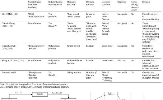
Table 1 (continued)
Supply Chain members involved
Differentiating New & Reman
Planning Horizon
Demand function
Decision variables
Objective Consi-dering obsoles-cence
Remark
Wu (2012b) [48] *OEM
*Remanufacturer Yes (Pn̸=Pr)
*Two period *Multi period
Linear in price
Prices *New *Reman
Max profit No Consider degree of
disassemblability
Chen & Chang (2013) [49]
Manufacturer Yes (Pn̸=Pr)
*Static *2-period *Multi periods over life-cycle
*Linear in price, with substi-tutable coefficient *Dynamic (over time)
Price of *New *Reman for each period
Max profit No *Static unconstrained *Dynamic pricing - constrained *Consider system of manufacturing only & hybrid settings
Jena & Sarmah (2013) [50]
*Remanufacturer *Retailer
Only reman product
Single period Random Cores price Max profit No Consider 3 schemes of collection: direct, indirect, coordinated
Xiong et al. (2013) [51] Manufacturer Only reman product
Finite & infinite horizon
Random Cores price Min cost No Consider lost sales and uncertain quality of used products
Proposed model *Manufacturer *Retailer *Collector
Yes
(Pn̸=Pr)
Selling horizon Function of time and price
Price of *Retail *Wholesale *Collecting
Max profit Yes Consider the impact of speed of change in demand
Note: Pn=price of new product, Pr=price of remanufactured product, Dn=demand of new product, Dr=demand of remanufactured product.
Fig. 1. Framework of the closed-loop pricing model.
2011. According to trial documents of Apple Inc. vs. Samsung Elec-tronics Co., Ltd [53], the sales of that product is entering decline phase starting on first quarter 2012.
After a certain period of time, some products reach their end-of-use and become the objects of end-of-used products collection. The end-of-used product would be acquired by collector under certain acquisition prices,Pc1andPc2, for product originated from IMG phases and
de-cline phase, respectively. The collected product is then transferred to manufacturer at pricePf, as the input for remanufacturing
pro-cess. The remanufactured product is sold to retailer at wholesale pricePrwand released to the market at retail pricePr.
The product considered in this model is single item, short life-cycle, with obsolescence effect after a certain period. Demand functions are time-dependent functions which represent the short life-cycle pattern along the entire phases of product life-cycle, both for new and remanufactured products; and linear in price.
There are four periods considered in this model, as depicted in
Fig. 2. In the first period
[
0,
t1]
, only new product is offered to themarket, while in second
[
t1, µ
]
and third period[
µ,
t3]
both new and remanufactured products are offered. The difference between second and third period is on the segments of life-cycle phases for both types. During second period, both new and remanufac-tured products are at the IMG phases. In the third period, the new product has entered the decline phase while remanufactured prod-uct has not. In the fourth period[t
3,
T]
, manufacturer has stoppedproducing new product and only offers remanufactured product which is assumed to be on the decline phase.
The market demand capacity is adopted from Wang and Tung [54] and extended to cover the obsolescence period, where
Fig. 2. Demand pattern of a product with gradual obsolescence, over time.
demand decreases significantly. The demand patterns are con-structed for both new and remanufactured product and the gov-erning functions are formulated as follows:
Dn
(
t)
=
Dn1
(
t)
=
U/
1+
ke−λUt
;
0≤
t≤
µ
Dn2
(
t)
=
U/ (λ
U(
t−
µ)
+
δ)
;
µ
≤
t≤
t3where k
=
U/
D0−
1δ
=
1+
ke−λUµ (3.1)Dr
(
t)
=
Dr1
(
t)
=
V/
1
+
he−ηV(t−t1)
;
t1≤
t≤
t3Dr2
(
t)
=
V/ (η
V(
t−
t3)
+
ε)
;
t3≤
t≤
Twhere h
=
V/
Dr0−
1ε
=
1+
he−ηV(t3−t1) (3.2)whereDn
(
t)
andDr(
t)
are demand pattern for new andremanu-factured products, respectively, as seen inFig. 2.Uis a parameter representing the maximum possible demand for new product,
µ
is the time when the demand reaches its peak, i.e. atUlevel.D0is
the demand at the beginning of the life-cycle (whent
=
0), andλ
is the speed of change in the demand as a function of time. A parallel definition is applicable forV,t3,Dr0, andη
respectively forthe remanufactured products. It is obvious thatDn
(
t)
andDr(
t)
arecontinuous at
µ
andt3, respectively, as shown inAppendix A.The new products are sold at retail pricePn1during
[
0, µ
]
, andPn2 during
[
µ,
t3]
. Since demand function is also linear in price,Fig. 3. Demand of new product during[0, µ]; (a) time-view (b) price-view.
at which demand would be zero. Remanufactured products are sold at retail pricePr during
[t
1,
T]
, and the maximum price isPn2, since customer would choose to buy new product rather than
remanufactured one when the remanufactured product price is as high asPn2. Therefore,
Demand of new product during
[
0, µ
] =
Dn1(
t)(
1−
Pn1/
Pm)
(3.3)Demand of new product during
[
µ,
t3] =
Dn2(
t)(
1−
Pn2/
Pm)
(3.4)Demand of reman product during
[t
1,
t3] =
Dr1(
t)(
1−
Pr/
Pn2)
(3.5)Demand of reman product during
[t
3,
T] =
Dr2(
t)(
1−
Pr/
Pn2).
(3.6)Fig. 3illustrates the demand of new product for the period of
[
0, µ
]
. The demand function information is shared to all members of the supply chain.Manufacturer decides the wholesale prices for new product
(
Pnw)
and remanufactured product(
Prw)
, retailer determines the retail prices(
Pn1,
Pn2,
Pr)
, while collector determines collectingprices Pc1 and Pc2 for cores collected from end-of-use product
within the periods of
[
0, µ
]
and[
µ,
t3]
respectively. Since theproduct has short life-cycle, remanufacturing process is only applied to cores originated from new products.
Return rate
(τ )
is an increasing function of the collecting price. We use the return rate function proposed by Qiaolun et al. [29], which was a result of their survey that employs a power function. The return rateτ
is defined on[t
1,
T]
and depends onPcas followsτ
=
γ
Pcθ (3.7)where
γ
are positive constant coefficients, andθ
∈ [
0,
1]
are expo-nents of the power functions, which determine curve’s steepness. It is assumed that collector only accepts cores with a certain quality grade, and all collected cores will be remanufactured.Since our research is focusing on pricing decision, we do not make an attempt to show detailed derivation of production and operational costs, and instead treat those costs as given parame-ters, which consist of unit raw material cost for new product
(
crw)
, unit manufacturing cost(
cm)
, unit remanufacturing cost(
cr)
, andunit collecting cost
(
c)
. The objective of the proposed model is to find the optimal prices that maximize profit, and we investigate two scenarios, (1) maximize profit independently, and (2) maxi-mize joint profit along the supply chain.4. Optimization
4.1. Independently optimized profit
4.1.1. Retailer’s optimization
In this scenario, manufacturer makes the first move by releasing initial wholesale prices
(
Pnw,
Prw)
. Retailer then optimizes theretail pricesPn1,Pn2, andPr. The profit function can be formulated
as follows:
ΠR
=
µ0
U
1
+
ke−λUt
1−
Pn1Pm
(
Pn1−
Pnw)
dt+
t3µ
U
λ
U(
t−
µ)
+
δ
1−
Pn2Pm
(
Pn2−
Pnw)
dt+
t3t1
V 1
+
he−ηV(t−t1)
1−
PrPn2
(
Pr−
Prw)
dt+
Tt3
V
µ
V(
t−
t3)
+
ε
1−
PrPn2
(
Pr−
Prw)
dt=
d1
1−
Pn1Pm
(
Pn1−
Pnw)
+
d2
1−
Pn2Pm
(
Pn2−
Pnw)
+
(
d3+
d4)
1−
PrPn2
(
Pr−
Prw)
(4.1)where
d1
=
1
λ
ln
δ
(
1+
k)
e−λUµ
d2=
1
λ
ln
λ
U(
t3−
µ)
+
δ
δ
d3
=
1η
ln
ε
(
1+
h)
e−ηV(t3−t1)
d4
=
1η
ln
η
V(
T−
t3)
+
ε
ε
.
The objective function is to maximize profit (4.1), and con-sequently it needs to satisfy the first derivative conditions
∂
ΠR/∂
Pn1=
0,∂
ΠR/∂
Pn2=
0, and∂
ΠR/∂
Pr=
0. The profitfunction(4.1)is not always concave along the considered interval, becausePn2took a hyperbolic form as a result of being the upper
bound ofPr, so we need to establish the interval on which profit
function is concave.
Property 1. The objective function
(
1)
is concave whenPn2
≥
3
(
d3+
d4)
PmPr2w 4d2.
(4.2)Proof. SeeAppendix B.
The above result implies that the demand of remanufactured product (d3andd4) influences the price of new product during the
decline stage. Demand capacity during decline stage which is af-fected by the length of that period has also contributed in shifting the interval of the concave function.
The optimal retail prices Pn1*, Pn2*, andPr* are obtained by
solving equations from first derivatives conditions:
Pn∗1
=
(
Pm+
Pnw) /
2 (4.3)Pr∗
=
(
Pn2+
Prw) /
2 (4.4)−
2 Pmd2
Pn∗2
3+
d2
1+
PnwPm
+
d3+
d4 4
Pn∗2
2−
(
d3+
d4) (
Prw)
2
FollowingProperty 1, Eq.(4.2)becomes the lower bound ofPn2.
It is expected thatP∗
n2is lower thanPn∗1to increase demand rate at
the decline stage, however the model allowsP∗
n2to attain higher
value thanPn∗1, which in turns is not attractive for customers. Our investigation showed thatPn2has a tendency to attain higher value
thanPn1, which is also consistent with Ferrer and Swaminathan’s
finding [37]. However, this is not an expected result since higher price during decline stage is not attractive for customers and might not be able to improve the demand rate. Therefore, we set a common price for new product,Pn1
=
Pn2. Retailer’s optimizationmodel becomes
Max
Pn,Pr
ΠR
=
(
d1+
d2)
1−
PnPm
(
Pn−
Pnw)
+
(
d3+
d4)
1−
PrPn
(
Pr−
Prw) .
(4.6)Decision variables: Pn: price of new product
Pr: price of remanufactured product
Parameters:
Pnw: wholesale price of new product
Prw: wholesale price of remanufactured product Pm: maximum price for new product
d1: total demand for new product within [0,
µ
]d2: total demand for new product within [
µ
,t3]d3: total demand for remanufactured product within [t1,t3]
d4: total demand for remanufactured product within [t3,T]
The existence of optimal pricesPn
,
Pr is shown inProperty 2,and the condition for obtaining prices that maximize retailer’s profit(4.6)is given inProperty 3. The optimal retail prices are given inProposition 1.
Property 2. There exists global extrema for profit maximization problem(4.6)in
{
(
Pn,
Pr)
|P
nw≤
Pn≤
Pm;
Prw≤
Pr≤
Pm;
Pn∈
R
,
Pr∈
R,
}.
Proof. SeeAppendix C.
Property 3. The objective function(4.6)is concave when
Prw 2
−
Pr+
d1+
d2d3
+
d4·
P3
n
Pm
>
0.
(4.7)Proof. SeeAppendix D.
Proposition 1. The optimal prices for optimization model(4.6)are P∗
nand Pr∗where
−
2(
d1+
d2)
Pm P
∗3
n
+
d1+
d2Pm
(
Pm−
Pnw)
+
d3+
d44
Pn∗2
−
d3+
d4 4 P2
rw
=
0 (4.8)Pr∗
=
P ∗n
+
Prw2
.
(4.9)Proof. SeeAppendix E.
FromProposition 1, we can observe that the optimal prices are not only determined by wholesale prices given by the manufac-turer, but also by the demand pattern imposed ind1,d2,d3, andd4,
which confirms the influence of demand patterns to the optimal retail prices.
4.1.2. Collector’s optimization
After retailer decides the optimal retail prices, collector then uses the resulting demand rates as the parameters in the profit
op-timization model, and the objective function is
Max
Pc
ΠC
=
γ
Pcθ(
d1+
d2)
1−
PnPm
Pf
−
Pc−
c
.
(4.10)Decision variables:
Pc: acquisition price for used product
Parameters:
Pn
,
Pm,
d1,
d2as mentioned earlierPf: transfer price of remanufacturable core from collector to re-manufacturer
γ
: constant coefficient of the return rateθ
: exponent of the return rate power functions c: unit collecting costProperty 4shows the existence of optimal pricePcfor collector’s
profit function(4.10). First derivative condition is applied to obtain the optimal collecting price as shown inProposition 2.
Property 4. There exists a global extrema for collector’s profit func-tion(4.10)in
Pc|
0≤
Pc≤
Pf;
Pc∈
R
.Proof. SeeAppendix F.
Proposition 2. The collector’s profit function(4.10)attains its maxi-mum in
Pc
|
0≤
Pc≤
Pf;
Pc∈
R
and the optimal collecting price is
Pc∗
=
θ
Pf
−
c
(θ
+
1)
.
(4.11)Proof. SeeAppendix G.
We assume balanced quantity throughout the supply chain, which is supported by Guide’s work [26]. Collector should only col-lect as much as the demand of the remanufactured product, which consequently determines transfer price.
Proposition 3. The optimal transfer price is
Pf∗
=
c+
θ
+
1θ
(
d3+
d4) (
1−
Pr/
Pn)
γ (
d1+
d2) (
1−
Pn/
Pm)
θ1.
(4.12)Proof. SeeAppendix H.
4.1.3. Manufacturer’s optimization
After observing retailer’s and collector’s prices, manufacturer determines the wholesale prices for both new
(
Pnw)
and reman-ufactured products(
Prw)
in order to maximize her profit which is expressed in the following objective function:Max
Pnw,Prw
ΠM
=
(
d1+
d2)
1−
PnPm
(
Pnw−
crw−
cm)
+
(
d3+
d4)
1−
PrPn
×
Prw
−
cr−
c−
θ
+
1θ
(
d3+
d4) (
1−
Pr/
Pn)
γ (
d1+
d2) (
1−
Pn/
Pm)
1θ
(4.13)
subject to the optimal prices of the retailer and collector. We apply Lagrange multipliers method, where we define Lagrangian func-tion associated with(4.13)as given in(4.14)
L
Pnw
,
Prw,
Pn,
Pr, ξ , ψ
=
ΠM+
ξ
−
2(
d1+
d2)
Pm
Pn3
+
d1
+
d2Pm
(
Pm−
Pnw)
+
d3+
d44
Pn2
−
d3+
d4 4 P2
rw
Pnw: wholesale price of new product
Prw: wholesale price of remanufactured product
Parameters:
Pn
,
Pr,
Pm,
d1,
d2,
d3,
d4,
Pf,
c, γ , θ
as mentioned earliercrw: unit raw material cost for producing new product cm: unit manufacturing cost for producing new product
cr: unit remanufacturing cost for producing remanufactured product
The first order conditions of the Lagrangian are regarded as the necessary conditions for the constrained optimization, and yield a nonlinear system. We treatPnandPras intermediary decision
vari-ables in this optimization problem sincePnandPr from retailer’s optimum pricing decisions are not expressed as explicit functions inPnwandPrw, hence the relations are expressed in the constraint functions.
Following Lagrange multiplier theorem [54], if there exist opti-mal wholesale pricesP∗
nw,Pr∗w,Pn∗,Pr∗, then they are the solutions
of first order conditions for(4.14), which are ∂∂ΠMP n
=
0,∂ΠM
∂Pr
=
0,∂ΠM
∂Pnw
=
0, ∂ΠM∂Prw
=
0, ∂ΠM∂ξ
=
0, and ∂ΠM∂ψ
=
0, that yields(4.15)to (4.20)respectively.1 Pm
(
d1+
d2) (
Pnw−
crw−
cm)
−
(
d3+
d4)
1−
PrPn
×
(
Prw−
cr−
c)
+
d3
+
d4γ (
d1+
d2) (
1−
Pn/
Pm)
1/θ×
(θ
+
1) (
d3+
d4)
1−
PrPn
1/θ−1P2
n
θ
2(
1−
Pn/
Pm)
×
(θ
−
1)
1−
PrPn
Pr
−
(θ
−
3)
×
PnPr Pm+
θ
Pr Pm−
P2
n
+
2Pr2Pm
+
6Pn2ξ
d1+
d2Pm
−
2Pnξ
d1+
d2Pm
(
Pm−
Pnw)
+
d3+
d44
−
ψ
=
0 (4.15)d3
+
d4Pn
Prw
−
cr−
c−
θ
+
1θ
(
d3+
d4) (
1−
Pr/
Pn)
γ (
d1+
d2) (
1−
Pn/
Pm)
1θ+
(
d3+
d4)
1−
PrPn
θ
+
1θ
2
×
(
d3+
d4) (
1−
Pr/
Pn)
γ (
d1+
d2) (
1−
Pn/
Pm)
1θ−1
−
2ψ
=
0 (4.16)Pm
−
Pn−
ξ
P2n=
0 (4.17)
1−
PnPm
−
ξ
Prw2
−
ψ
=
0 (4.18)−
2(
d1+
d2)
Pm
Pn3
+
d1
+
d2Pm
(
Pm−
Pnw)
+
d3+
d44
Pn2
−
d3+
d4 4 P2
rw
=
0 (4.19)2Pr
−
Pn−
Prw=
0.
(4.20)The second order conditions for the Lagrangian function, which re-flects the sufficient condition for a maxima, are not practical to be expressed analytically. Therefore, to ensure that the solution is a maxima we apply a numerical procedure to check the values of
profit numerically under an optimization search procedure.
4.2. Joint profit optimization
Under the joint profit scenario, all parties aim at maximum total profit along the supply chain. The joint profit function is summa-tion of retailer’s profit, collector’s profit, and manufacturer’s profit. Balanced quantity is also imposed in this model, and for remanu-factured product, the quantity of demand is equal to the quantity of returns, which also means collector only collects as much as the demand for remanufactured products. The optimization problem is given by the following expressions:
MaxΠJ
=
ΠR+
ΠC+
ΠM=
(
d1+
d2)
1−
PnPm
(
Pn−
Pnw)
+
(
d3+
d4)
1−
PrPn
(
Pr−
Prw)
+
γ
Pcθ(
d1+
d2)
1−
PnPm
Pf
−
Pc−
c
+
(
d1+
d2)
1−
PnPm
(
Pnw−
crw−
cm)
+
(
d3+
d4)
×
1
−
Pr Pn
Prw
−
Pf−
cr
(4.21)
s.t.
(
d3+
d4)
1−
PrPn
=
γ
Pcθ(
d1+
d2)
1−
PnPm
.
(4.22)
The joint profit function is then simplified to a function ofPn,
Pr, andPcas presented in Eq.(4.22). Considering balanced quantity
throughout the supply chain, then the optimization model for joint profit function becomes(4.23)
ΠJ
=
(
d1+
d2)
1−
PnPm
(
Pn−
crw−
cm)
+
(
d3+
d4)
×
1
−
Pr Pn
(
Pr−
cr−
Pc−
c)
(4.23)ΠJ
=
(
d1+
d2)
1−
PnPm
(
Pn−
crw−
cm)
+
(
d3+
d4)
1−
PrPn
(
Pr−
cr−
c)
−
(
d3+
d4)
×
1
−
Pr Pn
θ+θ1
γ (
d1+
d2)
1−
PnPm
−1θ.
(4.24)In finding the optimal prices, we assign first derivatives to zero
∂
ΠJ∂
Pn=
(
d1+
d2)
Pm
−
2Pn+
crw+
cmPm
+
(
d3+
d4)
Pr
−
cr−
cP2
n
−
(
d3+
d4)
1−
PrPn
θ+θ1×
γ (
d1+
d2)
1−
PnPm
−1θ×
θ
+
1θ
Pn(
Pn−
Pr)
−
1θ (
Pm−
Pn)
(
d1+
d2)
1−
Pn∗∗Pm
(
Pnw−
crw−
cm)
+
(
d3+
d4)
1−
Pr∗∗Pn∗∗
Prw
−
Pf−
cr
−
ΠRΠR
=
δ
ΠR
+
ΠM+
ΠC(4.28)
γ
P∗∗c
θ
1−
P∗∗nPm
Pf
−
Pc∗∗−
c
−
ΠCΠC
=
δ
ΠR
+
ΠM+
ΠC(4.29)
(
d1+
d2)
1−
Pn∗∗Pm
P∗∗
n
−
Pnw
+
(
d3+
d4)
1−
Pr∗∗Pn∗∗
P∗∗
r
−
Prw
−
ΠMΠM
=
δ
ΠR
+
ΠM+
ΠC(4.30)
Box I.
∂
ΠJ∂
Pr= −
1 Pn(
d3+
d4)
×
Pr−
cr−
c−
θ
+
1θ
(
d3+
d4)
1−
PrPn
γ (
d1+
d2)
1−
PnPm
1/θ
+
(
d3+
d4)
1−
PrPn
=
0 orPn
−
2Pr+
cr+
c+
θ
+
1θ
(
d3+
d4)
1−
PrPn
γ (
d1+
d2)
1−
PnPm
1/θ
=
0.
(4.26)The optimal values ofP∗∗
n andPr∗∗ that maximize joint profit are
obtained by solving Eqs.(4.24)and(4.25). Since we assume bal-anced quantity (consistent with Guide’s work [26]), the optimiza-tion model is reduced to a problem with two decision variables, PnandPr. These results only determine optimal retail prices, and
leave the wholesale prices (Pnw andPrw) and transfer price
(
Pf)
to be determined under coordinated decision policy, which incor-porate equal relative profit difference between independent and joint profit scenario between manufacturer and retailer. The inte-grated scenario accommodates coordinated pricing policy that en-sures higher (or might be lower) profit for each party, and makes this approach interesting for all members of the supply chain. The equal relative profit difference can be expressed as follows:
∆ΠR
ΠR
=
∆ΠMΠM
=
∆ΠCΠC
(4.27)
where∆ΠR
=
ΠR,J−
ΠR;∆ΠM=
ΠM,J−
ΠM;∆ΠC=
ΠC,J−
ΠC.Therefore, we get Eqs. (4.28)–(4.30)(seeBox I) where
δ
=
ΠJ
−
(
ΠR+
ΠM+
ΠC)
=
∆ΠR+
∆ΠM+
∆ΠC.This system of Eqs.(4.28)–(4.30)is solved forPnw
,
Prw, andPf to obtain the wholesale prices and transfer price under joint profit scenario.5. Numerical example and discussions
In this numerical example, the parameters in demand function are using data from numerical example in [54], because it repre-sents demand pattern of product with gradual obsolescence. How-ever, that study does not consider used product’s return, therefore parameters in return function is taken from numerical example in [29]. As for the cost parameters, we developed the data based on case studies in a report for Ellen MacArthur Foundation, Towards The Circular Economy [55].
New product’s demand capacity parameters areU
=
1000, D0=
90,λ
= [
0.
01,
0.
05,
0.
1,
0.
2]
, and remanufacturedprod-uct’s demand capacity parameters areV
=
500,Dr0=
50,η
=
[
0.
01,
0.
05,
0.
1,
0.
2]
. Selling horizon is divided into four time pe-riods wheret1=
1,µ
=
2,t3=
3, andT=
4. The unit rawmaterial cost for new productcrw
=
1500, unit manufacturingcostcm
=
1000, unit remanufacturing costcr=
800, and unit collecting costc=
100. Maximum price isPm=
12 000. Return rate parameters areγ
=
0.
01, andθ
=
0.
7. The decision variables arePn,
Pr,
Pnw,
Prw,
Pc,
Pf, which represent price of new product,price of remanufactured product, wholesale price of new product, wholesale price of remanufactured product, collection price and transfer price, respectively.Table 2presents the results.
From the results above, we have shown that joint profit scenario gives a higher total profit rather than optimized individually. It is also interesting to note that the joint profit model accommodates coordinated pricing policy that ensures higher profit for each party, and making this approach interesting for all members of the supply chain. Demand rate in the joint profit scenario is much higher than in the independent one, even though it came from the same demand parameters. In the independent model, with the lack of integrated decision among the three players, the retail prices were set substantially higher than the true optimums. We also observed that Collector profit is much lower than Retailer’s and Manufacturer’s, because Collector only gains from remanufactured product. This result is consistent with Qiaolun’s [29].
The optimization models also show that transfer price can be found by balancing the return rate with the demand of remanu-factured product. Under this approach we can determine trans-fer price that could benefit both manufacturer and collector, and it puts collector at better position rather than the presumed con-dition that transfer price is negotiated between manufacturer and collector. Since manufacturer is the Stackelberg leader, it is pos-sible that collector would have been in lower bargaining position. Even though this approach might not be interested for the manu-facturer, as it puts limitation to manufacturer’s power, but it actu-ally creates sustainability for the overall closed-loop supply chain. The betterment in collector’s position would be a good motivation to continue collecting used products for remanufacturing, and sup-port environment protection.
Different speeds of change in the demand of new and reman-ufactured product obviously result in different pricing decisions. However, faster penetration to the market, which is shown by the higher speed of change in demands, does not simply generate higher total profits. It can be seen from the demand function and optimization models that speed of change in demand will influence the sales volumes in each period and subsequently has impacted the optimum pricing decision. As stated inPropositions 1and3, the optimal prices depend on the demand volumes in respective periods. We can also find an interval of speed of change in demand where the total profit reaches its highest value. This could lead to a marketing decision where the players should control market pen-etration such that the speed of change is within the desirable in-terval.
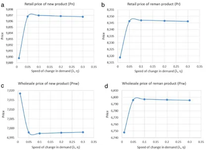
The impact of demand’s speed of change to the optimal prices
In this paper, demand of short life-cycle product is time-dependent and demand pattern over time is influenced by several parameters, such as speed of change in demand as shown in(3.1)
Comparison between independent and joint profit scenarios.
λ, η
0.01 0.05 0.10 0.20
Independent scenario
Pn 9,889.78 9,896.80 9,896.98 9,896.86
Pr 8,318.83 8,346.32 8,347.02 8,346.56
Pnw 7,018.45 6,997.86 6,997.33 6,997.68
Prw 6,747.80 6,795.85 6,797.06 6,796.26
Pc 422.04 468.28 469.50 468.70
Pf 1,124.96 1,237.25 1,240.21 1,238.27
ΠM 2,391,233.07 2,453,199.12 2,443,651.42 2,434,076.99
ΠR 1,246,142.45 1,279,206.64 1,274,245.91 1,269,241.66
ΠC 145,869.03 176,221.10 176,253.30 175,094.89
Total profit 3,783,244.55 3,908,626.86 3,894,150.63 3,878,413.54
Joint profit scenario
Pn 7,816.53 7,837.87 7,838.40 7,838.06
Pr 4,720.08 4,758.91 4,759.89 4,759.25
Pnw 5,756.12 6,110.48 6,115.01 6,579.60
Prw 4,133.21 3,566.64 3,560.95 2,742.55
Pc 297.96 321.15 321.74 321.36
Pf 913.79 1,004.01 1,006.38 1,004.83
ΠM,J 3,178,657.26 3,248,364.50 3,235,368.72 3,222,922.56
ΠR,J 1,656,492.54 1,693,841.07 1,687,088.16 1,680,582.67
ΠC,J 193,903.16 233,340.36 233,357.51 231,840.36
Total profit 5,029,052.96 5,175,545.93 5,155,814.39 5,135,345.59
Table 3
Optimal prices under various speeds of change in demand.
λ, η Pn Pr Pnw Prw ΠM ΠR ΠC
0.01 9890 8319 7018 6748 1,246,142.45 2,391,233.07 145,869.03
0.05 9897 8346 6998 6796 1,279,206.64 2,453,199.12 176,221.10
0.1 9897 8347 6997 6797 1,274,245.91 2,443,651.42 176,253.30
0.2 9897 8347 6998 6796 1,269,241.66 2,434,076.99 175,094.89
0.3 9897 8346 6998 6796 1,266,865.91 2,429,539.87 174,376.30
during IMG phases, and decreases during decline phase. Therefore, the accumulation of demand over time would influence the optimal prices, since we consider the whole product life cycle. We vary
λ
andη
to study their impacts on decision variables and the objective functions.Table 3andFig. 4show the results.As shown inFig. 4, optimal prices are sensitive to parameters that reflect the speed of change in demand for lower market penetration, but they are robust for higher speed of change in demand. This can be explained by the specific nature of demand pattern. For a short life cycle product with demand pattern as given in(3.1)and (3.2), higher speed of change in demand leads to a condition that is closer to constant demand. Therefore, optimal prices do not change significantly compared to the ones with lower speed of change in demand. This situation is applicable to a product with demand pattern such that in the beginning of product’s introduction phase, the increase in demand tends to be very steep, such as launching a new model of smartphone. After a certain time period, the demand decreases quite rapidly. We argue that the optimal prices are more robust in higher speed, because the effect of speed of change becomes less significant. This means, when speed of change in demand is high such that the sales reach maximum demand in a very short time, then the price setting does not need to be adjusted when there is a small change in the speed. However, when the speed is low, the sales climb up rather slowly to reach maximum demand, so it is important to adjust price setting when there is a change in the speed, to avoid sub-optimal prices.
The managerial insight for this matter can be explained as fol-lows. Under lower speed of change in demand, decision makers need to carefully update the prices to avoid sub-optimality. But when it moves fast to the peak, price updates become less urgent, since the demand has reached its uniform pattern.
6. Conclusion and future research agenda
In this study we have developed pricing decision models for remanufacturing of short life-cycle product. The study fills the gap of remanufacturing literature which to date has been mostly dominated by durable products. For some short life cycle products, remanufacturing is a sensible activity to do, but the speed of collecting and remanufacturing the used products should be quick as the demand for the product is diminishing fast. Here are some conclusions that we obtain from this study:
•
Reducing the price of new products during the decline phase does not give better profit for the whole system,•
The total profit obtained from optimizing each player indepen-dently is lower than the total profit of the integrated model where we optimize the joint profit for three members in the supply chain, namely manufacturer, retailer and collector. None of the player is worse off by moving from the independent model to the joint profit model, under coordinated pricing policy,•
The total demand is significantly higher under the integrated model. This is understandable because the retail prices are lower for both the new and remanufactured products. The lack of coordination in making the pricing decision has led the inde-pendent models to set high retail prices and hence the demand potential is not well exploited,Fig. 4. Optimal prices charts under various speeds of change in demand.
•
When demand penetration is low, small changes in the demand rate affect price settings substantially. However, when demand penetration is high, price decision is robust against the change in demand rate.Future research may be directed toward development of models that consider different demand processes, multiple objective func-tions, and the case when balanced quantity is not the case. It may be possible that the collector is not able to collect at the quantity desired by the manufacturer. It is also possible that the manufac-turer has a certain capacity constraint where not all demand can be satisfied. In such as case it is important to take into account the service level.
Appendix A. Dn
(
t)
and Dr(
t)
are continuous atµ
and t3,respectively
Dn1
(µ)
=
U 1
+
ke−λUµDn2
(µ)
=
U
(λ
U(µ
−
µ)
+
δ)
=
U
δ
=
U
1
+
ke−λUµ
×
Dn1(µ)
=
Dn2(µ)
lim
t→µ−Dn
(
t)
=
t→limµ−U 1
+
ke−λUt=
U 1
+
ke−λUµlim
t→µ+Dn
(
t)
=
t→limµ+U
(λ
U(
t−
µ)
+
δ)
=
U 1
+
ke−λUµ
×
limt→µ−Dn
(
t)
=
t→limµ+Dn(
t).
Therefore Dn
(µ)
=
limt→µDn(µ)
=
1+keU−λUµ→
Dn(
t)
iscontinuous att
=
µ
.Similarly,
Dr1
(
t3)
=
V 1
+
he−ηV(t3−t1)Dr2
(
t3)
=
V
(η
V(
t3−
t3)
+
ε)
=
Vε
=
V 1
+
he−ηV(t3−t1)
×
Dr1(
t3)
=
Dr2(
t3)
lim
t→t3−
Dr
(
t)
=
lim t→t−3V
1
+
he−ηV(t−t1)=
V 1
+
he−ηV(t3−t1i)lim
t→t3+
Dr
(
t)
=
lim t→t+3V
(η
V(
t−
t3)
+
ε)
=
V1
+
he−ηV(t3−t1)
×
limt→t3−
Dr
(
t)
=
lim t→t3+Dr
(
t).
ThereforeDr
(µ)
=
limt→t3Dr(
t3)
=
V1+he−ηV(t3−t1)
→
Dr(
t)
is continuous att=
t3.Appendix B. Proof ofProperty 1
ΠR
=
d1
1−
Pn1Pm
(
Pn1−
Pnw)
+
d2
1−
Pn2Pm
(
Pn2−
Pnw)
+
(
d3+
d4)
1−
PrPn2
(
Pr−
Prw)
∂
2ΠR
∂
Pn21= −
2d1Pm
<
0
∂
2ΠR∂
P2n1
∂
2ΠR∂
Pn1∂
Pn2∂
2ΠR
∂
Pn2∂
Pn1∂
2ΠR
∂
P2n2
=
2d1 Pm
d2Pm
+
2(
d3+
d4)
Pr(
Pr−
Prw)
Pn22
|H| =
∂
P2n1
∂
Pn1∂
Pn2∂
Pn1∂
Pr∂
2ΠR
∂
Pn2∂
Pn1∂
2ΠR
∂
Pn22∂
2ΠR
∂
Pn2∂
Pr∂
2ΠR∂
Pr∂
Pn1∂
2ΠR∂
Pr∂
Pn2∂
2ΠR∂
P2nr
=
2d1(
d3+
d4)
PmPn2
(
d3+
d4)
Pr2w P3n2
−
4d2 Pm
≤
0Since
|H
1| =
∂
2ΠR/∂
Pn21<
0; and|H
2| =
(∂
2ΠR/∂
Pn21)(∂
2ΠR/∂
Pn22)
−
(∂
2ΠR
/∂
Pn1∂
Pn2)
2>
0, then forΠR to be a concave function,|H
3| = |H|
should be less than or equal to zero. Therefore
(
d3+
d4)
Pr2w Pn32−
4d2
Pm
≤
0or
Pn2
≥
3
(
d3+
d4)
PmPr2w 4d2.
Appendix C. Proof ofProperty 2
SinceΠRis a two-variable rational function with a rational
pa-rameter in the coefficients, then it is discontinuous whenPm
=
0andPn
=
0. However,Pmis a nonzero parameter, andPnw≤
Pn≤
Pmwith positivePnw, thereforeΠRis continuous in
{
(
Pn,
Pr)
|P
nw≤
Pn≤
Pm;
Prw≤
Pr≤
Pm;
Pn∈
R,
Pr∈
R,
}
. SinceΠRiscontinu-ous in a closed interval then it attains global extrema there.
Appendix D. Proof ofProperty 3
∂
ΠR∂
Pn=
d1+
d2 Pm(
Pm+
Pnw−
2Pn)
+
d3
+
d4P2
n
Pr2
−
PrwPr
∂
2ΠR
∂
P2n
= −
2d1+
d2c
−
2d3
+
d4P3
n
Pr
(
Pr−
Prw) <
0∂
ΠR∂
Pr=
d3+
d4 Pn(
−
2Pr+
Prw+
Pn)
∂
2ΠR
∂
P2r
= −
2d3+
d4 Pn<
0∂
2ΠR
∂
Pn∂
Pr=
∂
2Π
R
∂
Pr∂
Pn=
d3+
d4 P2n
(
2Pr−
Prw)
D
=
∂
2Π
R
∂
P2n
·
∂
2ΠR
∂
P2r
−
∂
2ΠR
∂
Pn∂
Pr
2=
4(
d1+
d2) (
d3+
d4)
PmPn−
(
d3+
d4)
2
P4
n
(
2Pr−
Prw)
2>
04
(
d1+
d2)
Pm
−
(
d3+
d4)
P3n
(
2Pr−
Prw)
2>
02Pr
−
Prw<
4d1
+
d2 d3+
d4·
P3
n
Pm
Prw 2
−
Pr+
d1+
d2d3
+
d4·
P3
n
Pm
>
0.
Appendix E. Proof ofProposition 1
The critical points for (4.6) are obtained by applying first derivatives condition,
∂
Pr=
Pn(
−
2Pr+
Prw+
Pn)
=
0−
2Pr+
Prw+
Pn=
0→
Pr∗=
Pn∗
+
Prw 2∂
ΠR∂
Pn=
d1+
d2 Pm(
Pm+
Pnw−
2Pn)
+
d3+
d4 P2n
Pr2
−
PrwPr
=
0−
2(
d1+
d2)
Pm
Pn∗3
+
d1+
d2 Pm(
Pm−
Pnw)
Pn∗2+
(
d3+
d4)
Pn∗
+
Prw 2
Pn∗
+
Prw 2−
Prw
=
0−
2(
d1+
d2)
Pm
Pn∗3
+
d1
+
d2Pm
(
Pm−
Pnw)
+
d3+
d44
Pn∗2
−
d3+
d4 4 P2
rw
=
0.
From Property 4, the retailer profit function is concave when condition(4.7)is satisfied, therefore
Prw
2
−
Pr+
d1
+
d2d3
+
d4·
P3
n
Pm
>
0Prw 2
−
Pn
+
Prw 2+
d1+
d2d3
+
d4·
P3 n Pm
>
0 Pn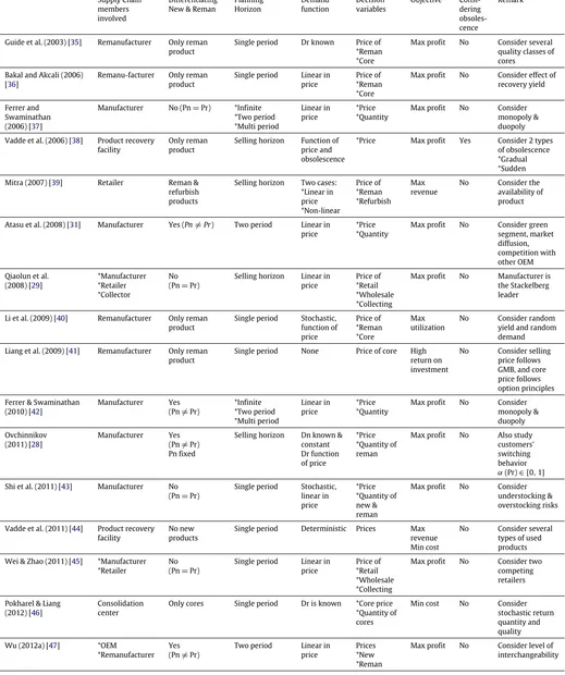
![Fig. 3. Demand of new product during [0, µ]; (a) time-view (b) price-view.](https://thumb-ap.123doks.com/thumbv2/123dok/1561315.2049906/5.595.311.564.223.450/fig-demand-new-product-time-view-price-view.webp)