Athena Scientific, Belmont, Massachusetts

Introduction to Probability

SECOND EDITION

Dimitri

P.

Bertsekas and John N. Tsitsiklis

Massachusetts Institute of Technology

WWW site for book information and orders

http://www.athenasc.com

7

Markov Chains

Contents

7. 1 . Discrete-Time Markov Chains

7.2. Classification of States . . . .

7.3. Steady-State Behavior . . .

.

7.4. Absorption Probabilities and Expected Time to Absorption

7.5. Continuous-Time Markov Chains

7.6. Summary and Discussion

Problems . . . .

·

p. 340

·

p. 346

·

p. 352

·

p. 362

·

p. 369

·

p. 378

·

p. 380

340 Markov Chains Chap. 7

The Bernoulli and Poisson processes studied in the preceding chapter are memo­

ryless, in the sense that the future does not depend on the past : the occurrences

of new �:successes" or ':arrivals" do not depend on the past history of the process.

In this chapter, we consider processes where the future depends on and can be

predicted to some extent by what has happened in the past.

We emphasize models where the effect of the past on the future is sum­

marized by a

state.

which changes over time according to given probabilities.

We restrict ourselves to models in which the state can only take a finite number

values and can change according to probabilities that do not depend on the time

of the change. We want to analyze the probabilistic properties of the sequence

of state values.

The range of applications of the type of models described in this chapter

is truly vast. It includes just about any dynamical system whose evolution over

time involves uncertainty, provided the state of the system is suitably defined.

Such systems arise in a broad variety of fields, such as. for example. commu­

nications. automatic control, signal processing. manufacturing, economics. and

operations research.

7. 1

DISCRETE-TIME MARKOV CHAINS

We will first consider

discrete-time Markov chains,

in which the state changes

at certain discrete time instants, indexed by an integer variable

n .

At each time

step

n,

the state of the chain is denoted by

Xn .

and belongs to a

finite

set S of

possible states, called the

state space.

Without loss of generality, and unless

there is a statement to the contrary. we will assume that S

=

{ I,

.

.

.

.

m

}

,

for some

positive integer

m.

The Markov chain is described in terms of its

transition

probabilities

Pij :

whenever the state happens to be

i,

there is probability

Pij

that the next state is equal to

j .

:Mathematically.

Pij

=

P(Xn+l

=

j I

Xn

=

i).

i.

j

E

S.

The key assumption underlying Markov chains is that the transition probabilities

Pij

apply whenever state

i

is visited, no matter what happened in the past, and

no matter how state

i

was reached. J\lathematically, we assume the

Markov

The transition probabilities

Pij

must be of course nonnegative, and sum to

one:

m

Sec. 7. 1 Discrete-Time Markov Chains 341

We will generally allow the probabilities

_Pii

to be positive, in which case it is

possible for the next state to be the same

as

the current one. Even though the

state does not change, we still view this

as

a state transition of a special type (a

"self-transition" ) .

Specification of Markov Models

•

A Markov chain model is specified by identifying:

(a) the set of states S

=

{I,

.

.

.

, m},

(b) the set of possible transitions, namely, those pairs

(i,

j) for which

Pij

> 0, and,

(c) the numerical values of those

Pij

that are positive.

•

The Markov chain specified by this model is a sequence of random

variables

XO, X1 , X2, .

. .

, that take values in S, and which satisfy

P(Xn+1

=

j

I Xn

=

i,

Xn-l

=

in-I , . . . , Xo

=

io)

=

Pij ,

for all times

n,

all states i, j

E

S, and all possible sequences

io,

. .

.

, in- l

of earlier states.

All of the elements of a Markov chain model can be encoded in a

transition

probability matrix,

which is simply a two-dimensional array whose element

at the ith row and jth column is

_{Pij :}

Pl l Pl2

Plm

P21 P22

P2m

Pml pm2

Pmm

It

is also helpful to lay out the model in the so-called

transition probability

graph,

whose nodes are the states and whose arcs are the possible transitions.

By recording the numerical values of

_Pij

near the corresponding arcs, one can

visualize the entire model in a way that can make some of its major properties

readily apparent.

Example 7.1 . Alice is taking a probability class and in each week, she can be

either up-to-date or she may have fallen behind. If she is up-to-date in a given week, the probability that she will be up-to-date (or behind) in the next week is

Pi l

=

0.8.

P12

=

probability is

P21

=

[�:� 0.4] '

graph is show n in 7. 1 .

7 . 1 : The transition

7

P22

=

0.4,

in 7. 1 .

7 . 2 . A fly moves along

a

line i n u nit

increments. At t ime

p

eriod,

it

move

s

one unit to the left with

p

robabiHty

0.3,

one unit to the right with probability 0.3, and stays i n p lace with probabiHty

i

nd

ep

end

e

nt the

movements.

spiders are

at

positions 1 and m: if it is captured by a and the

terminates. We want to construct a Markov chain model, assuming that the fly starts in a position between 1 m.

us states 1 , 2 , . . . , m , with positions of the fly. The nonzero transition probabilities are

{

0.31

Pi] ::::::: 0.4,

Pu

::::::: 1 , pmm ::::::: I , if j = i - l or j = i

+

1 ,

if j = i, for i ::::::: 2 , . .. , m - 1 .

matrix are in

7.2: The t ransi tion probability and the transi tion

7.2, for the case where m = 4.

ma-7. 1

State 1 :

with

2:

Machine is

is

in

two states:

[

1 - b b

]

.

r 1 - r

1 b

7. 3: 1tansition

b

T broken

1 'r

for 7.3 .

7 . 4 : _{Transition probabi lity graph for t he second part of Exam ple 7.3. A}

machine that has remained broken for e = 4 days is replaced by a new, working machine.

models. In

=

io,

Xl = il ,

_{. . .}

I

To verify t his property, note that

P(Xo = io , = il }

. . .

� Xn ==

)

==

io, · . .

I

Xn- 1

== in - l

, . . . � 1

== in- l

)

,

we have

apply

7

same argument to the term P(Xo == - 1 ) and continue similarly,

we eventually the state

Xo

is

p (X 1 == i

1 ,

. . . • X n == I X 0

==

io ) ₌₌

Graphically, a state _{sequence can be identified with a sequence of arcs in the}

transition probability and the such a the

IS by of arcs

traversed by the

We

7.4. For I we

P ( Xo

=

2� Xl

=

2.

=

2 ,

= 3, X4 = =

to a of is no

Sec. 7. 1 Discrete-Time Markov Chains 345 n-Step Transition Probabilities

Many Markov chain problems require the calculation of the probability law of

the state at some future time, conditioned on the current state. This probability

law is captured by the

n-step transition probabilities,

defined by

Tij (n)

=

P (Xn

j

I

Xo

=

i).

In words,

Tij (n)

is the probability that the state after

n

time periods will be j,

given that the current state is

i.

It can be calculated using the following basic

recursion, known as the

Chapman-Kolmogorov equation.

Chapman-Kolmogorov Equation for the n-Step Transition Probabilities

The n-step transition probabilities can be generated. by the recursive formula

m

T

i

j

(

n

)

=

L

_Ti

k(

n

- I)Pkj ,

k=l

starting with

for n

>

1 ,

and all i, j,

To verify the formula, we apply the total probability theorem as follows:

m.

probability

Pkj

of reaching j at the next step.

We can view

Tij (n)

as the element at the ith row and jth column of a two­

dimensional array, called the

n-step transition probability matrix.

t

Fig­

ures

7.6

and

7.7

give the n-step transition probabilities

Tij (n)

for the cases of

t Those readers familiar with matrix multiplication, may recognize that the

Chapman-Kolmogorov equation can be expressed

as

follows: the matrix of n-step tran­

sition probabilities

TtJ

(n) is obtained by multiplying the matrix of (n - I)-step tran­

sition probabilities

T

ik

(n

- 1 ) ,

with the one-step transition probability matrix. Thus,

7.5: Deriva.tion of the

at state j at time n is the sum of the

Chap. ₇

probability T,k (n - l )Pkj of the different ways of _{j .}

on

ity of being

rij (n)

7.6, we see

this l imit does not depend Furthermore, the probability initial state i n is but over time this

(but by no means all)

a

7.7, we see a qualitatively different behavior: (n)

on the initial can zero for states. Here, we that are "absorbing," sense that they are infinitely

once are states 1 4 to

capture of the fly by one of the two spiders. Given enough time: it is certain that some absorbing state will Accordingly: probability of being at the

2

a

we start to that These examples

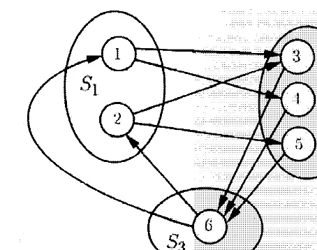
CLASSIFICATION STATES

are

this is the subject of the

some

some

7.6: n-step transition probabi lities for the "up-to-date/behind" Exam-ple 7. 1 . Observe that as n (n) converges to a limit that does not depend on the initial state i .

once, are not be the case. which this occurs .

t o b e visited again, while In this section, we focus on the

we wish to classify

of a Markov chain with a _focus on the freq uency with which are

As a a us

that a state

j

is from a state i _{if for some the n-step} transition

probabi_lity _Tij

(n)

, if is positive probability of _{j ,} starting from

i,

a_fter some _of time periods.

An

definition

is t hat is a possible _{1-, 1 1 1} . .

.

, h

j,

starts at i

more

(i, id , (il ,

, in-l ), (in- l , j)

Let

A( i)

be the set _of are accessible from i. We if for j that is from i, i is also

all j belong to

A(i)

_we i to

A(j).

i, we can only visit states j E

i

and, given enough ir a

an infinite number times.

version of argument .

)

is it is to

end-of-chapter problems for a

:L ;3 <\

o

7.7: shows n-step transit ion probabilities

7.2. These are the of

reach-from state i. We observe t hat probabilit ies converge to a limit, hut the l i m i t on the state. I n this

note t hat the Ti 2 (n) and Tz3 (n) of

2 or 3\ go to zero! as n i ncreases .

if is a state j E

AU)

t

hat i is from j .

7

state i . there is positive that the state enters such a j . Given enough this win happen, and i cannot be after that . Thus, a transient

state will

only

be _{visited a} finite number see

the

or rec

u

rrence is arcs of t

ran-[

t

h

ose

p

airs (i, w

h

ich

Pij

>

0]

and not the

7.8 provides an example of a transition

prob-a recurrent stprob-ate, the set are �

form

a

(or

simply

that states

in A (

i) are all

from no state A ( i ) is from t

h

em.

lvlathematically, for a recurrent state _i, we have A ( i ) = A (j ) for all j that belong

to

A( i) !

as can seen from recurrence. In

of 7.8, sta

t

es 3 a class, and s

t

ate 1 itself also forms a

7. 2 of

gIven

7.8: Classification of states given the t ransition probabi lity S

tart-from state I , the accessi_ble state is itself. and so 1 is a recu rrent state.

States 1 . 3, and 4 are accessible from 2. but 2 is not accessihle from an:v' of them,

so state 2 is transient . States 3 and 4 are accessible from each other . and are both recurrent .

probleIn . It follow::; that must exist at one recurrent

at one elM!:). the fonowing conclusion.

• A Markov can be decomposed into one or more recurrent classes,

•

•

•

possibly some states.

recurrent state is

is not

states

possibly state.

recurrent states are

7.9 �,Iarkov

1S

from

a

provides a powerful concept ual tool for reasoning about I\.farkov chains of

Hnmber of times:

For the

purpose of

behavior of

it

is

iIn-to analyze chains _that consist of a recurrent class. For the

it is t o

particul

a

r class o f recu_rrent

states is

entered

given transient state. These two issues. and

1.9: of l\·farkov chain into recurrent classes and transient states.

if 1- > 1 .

is

if k

=

1 . . . . . d

i f k =

1 .

7.2

Figure 7. 10: Structure of a periodic recurrent class. I n t his example . d = 3.

Thus. in a periodic recurrent

in order,

d

recurrent

w_e nlove through the sequence

in the same s ubset

.

As an example,

7.9 1 2) is

the same is true of the class third chain of Fig.

All

ot her

reason is that from i . n .

The

a way to verify aperiodicity of a recurrent whether

there a special n � 1 and a special i E R from which all states

in

R

can (n) >

0

for an j E an consider

the first chain in from state I I every state is possi ble at time

n = 3, SO unique recurrent of t hat is

A converse

a recurrent

for 'l

•

(

or to _S 1 if k =

d).

R.

turns out to be true: if n

such

Tij (n)

>

0

be group_ed in _d

from to

1

• The class is if and only if a

352 Markov Chains Chap. 7

7.3 STEADY-STATE BEHAVIOR

In Markov chain models, we are often interested in long-term state occupancy

behavior, that is, in the n-step transition probabilities

Tij (n)

when n is very

large. We have seen in the example of Fig.

7.6

that the

Tij (n)

may converge

to steady-state values that are independent of the initial state. We wish to

understand the extent to which this behavior is typical.

If there are two or more classes of recurrent states, it is clear that the

limiting values of the

Tij (n)

must depend on the initial state

(

the possibility of

visiting

j

far into the future depends on whether

j

is in the same class as the

initial state

i).

We will, therefore, restrict attention to chains involving a single

recurrent class, plus possibly some transient states. This is not as restrictive

as it may seem, since we know that once the state enters a particular recurrent

class, it will stay within that class. Thus, the asymptotic behavior of a multiclass

chain can be understood in terms of the asymptotic behavior of a single-class

chain.

Even for chains with a single recurrent class, the

Tij (n)

may fail to converge.

To see this, consider a recurrent class with two states,

1

and 2, such that from

state

1

we can only go to 2, and from 2 we can only go to

1 (P12

=

P21 = 1 ).

Then,

starting at some state, we will be in that same state after any even number of

transitions, and in the other state after any odd number of transitions. Formally,

Tii (n) =

{

1,

j

approaches a limiting value that is independent of the initial state

i,

provided

we exclude the two situations discussed above

(

multiple recurrent classes and

/

or

a periodic class

)

. This limiting value, denoted by

7r j ,

has the interpretation

7rj �

P(Xn

=

j),

when n is large,

and is called the

steady-state probability of j.

The following is an important

theorem. Its proof is quite complicated and is outlined together with several

other proofs in the end-of-chapter problems.

Steady-State Convergence Theorem

Consider

a Markov chain with

a

single recurrent class, which is

aper

i

od

ic.

Sec. 7.3 _{Steady-State Behavior}

(a) For each j, we have

lim

Tij (n)

=

1r'j ,

n-oo

for all

i.

(b) The

1r'j

are the unique solution to the system of equations below:

(c) We have

The steady-state probabilities

1l'j

sum to

1

and form a probability distri­

bution on the state space, called the

stationary distribution

of the chain.

The reason for the qualification "stationary" is that if the initial state is chosen

according to this distribution, i.e.! if

P(Xo

=

j)

1l'j .

j

= 1 , .. . , m,

then, using the total probability theorem, we have

m m

P(XI

=

j )

L

P(Xo

=

k)Pkj

=

L

1l'kPkj

=

1l'j ,

k=l

k=l

where the last equality follows from part (b) of the steady-state convergence

theorem. Similarly, we obtain

P(Xn

j)

=

1l'j ,

for all n and j . Thus, if the

initial state is chosen according to the stationary distribution, the state at any

future time will have the same distribution.

The equations

m

1l'j

L

1l'kPkj ,

j

= 1 , . . . , m,

k=l

are called the

balance equations.

They are a simple consequence of part (a)

of the theorem and the Chapman-Kolmogorov equation. Indeed, once the con­

vergence of

Tij (n)

to some

1l' j

is taken for granted, we can consider the equation,

m

354 Markov Chains Chap. 7

the balance equations can be solved to obtain the

7rj .

The following examples

illustrate the solution process.

Example

7.5. Consider a two-state Markov chain with transition probabilities

PI I =

0.8,

This is a generic property, and in fact it can be shown that any one of the balance equations can always be derived from the remaining equations. However, we also know that the 7rj satisfy the normalization equation

7rl

+

7r2 =

1,

which supplements the balance equations and suffices to determine the 7rj uniquely. Indeed, by substituting the equation 7rl = 37r2 into the equation 7rl

+

7r2 = 1 , we obtain 37r2

+

7r2 = 1 , or

7r2 =

0.25,

which using the equation 7rt

+

7r2 = 1 , yields

7rl =

0.75.

This is consistent with what we found earlier by iterating the Chapman-Kolmogorov equation (cf. Fig.

7.6).

so

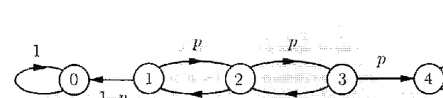
1. 1 1 : _Transition

1f) =

( 1

1

355

wet

states:

1 , 2 .

for 7.6.

0 < p <

1)

are

+

p1r2 , 1f2 = 1fo + ptrl .

1

1fo 1f t = -- ,

I1 J 1' ,j DonI' 3

Door _.J

7,,12: Transition in for the case of

m = 5 doors. that 0 < p < 1 1 it is not initial every state j can be reached in

to see t hat an and t herefore the

on some

m states:

i, i = 1, _.

.

_{. , m.}

o

I - p

o

p

1fl = ( 1

-p

0 0

o

p

0 1 p O p

o o 0

7T1 = p1f'i- l

+ (1

7T

Tn. = + p1f'Tn. 1 .

is

o o o

I - p 1

-o o

o

1, = . . • , m - 1 ,

once we

7.

7

Sec. 7.3 Steady-State Behavior 357

should have the same steady-state probability. This suggests the solution

j = 1 , . . . , m.

Indeed, we see that these 'Trj satisfy the balance equations as well as the normal­ ization equation, so they must be the desired steady-state probabilities (by the uniqueness part of the steady-state convergence theorem) .

Note that i f either

p =

0 or

p =

1 , the chain still has a single recurrent class but is periodic. In this case, the n-step transition probabilities Tij (n) do not converge to a limit, because the doors are used in a cyclic order. Similarly, if m is even, the recurrent class of the chain is periodic, since the states can be grouped into two subsets, the even and the odd numbered states, such that from each subset one can only go to the other subset.

Long-Term Frequency Interpretations

Probabilities are often interpreted as relative frequencies in an infinitely long

string of independent trials. The steady-state probabilities of a Markov chain

admit a similar interpretation, despite the absence of independence.

Consider, for example, a Markov chain involving a machine, which at the

end of any day can be in one of two states, working or broken down. Each time

it breaks down, it is immediately repaired at a cost of

$ 1 .

How are we to model

the long-term expected cost of repair per day? One possibility is to view it as the

expected value of the repair cost on a randomly chosen day far into the future;

this is just the steady-state probability of the broken down state. Alternatively,

we can calculate the total expected repair cost in

n

days, where

n

is very large,

and divide it by

n.

Intuition suggests that these two methods of calculation

should give the same result. Theory supports this intuition, and in general we

have the following interpretation of steady-state probabilities (a justification is

given in the end-of-chapter problems) .

Steady-State Probabilities

as

Expected State Frequencies

For a Markov chain with a single class which is aperiodic, the steady-state

probabilities

7r j

satisfy

1.

Vij(n)

7rj

=

1m

,

n--+oo n

where

Vij

(n)

is the expected value of the number of visits to state j within

the first

n

transitions, starting from state

i.

be

from j as the long-term fraction of transitions

Chap. 7

move the

Expected of a Particu1ar Transition

lim

n - oo _n

with a single class which is

(n)

k.

the frequency interpretation of 7r j equation

m

k= l

has an intuitive meaning.

It

expresses the fact that the expected frequency 7fj

of to j sum the 1rkPkj of

of the balance in terms of In

a very nu mber of transitions, we expect a fraction 1TkPkj that bring t he state

from k to j. (This also to transitions from j to which occur with

.) The sum of the expected of such transitions is the

of at state j.

t I n fact , some stronger statements are also true, such as the following. Whenever

we carry out a probabilistic experiment and a trajectory of the Markov chain state j is t he observed long-term transitions

Even though the trajectory is random,

which

a

intro-duces some generic notation for the transition probabilit ies

.

In particular,

l = i + l l

l = i - l l

( "birth" probability at

(

probability at

7.14: Transition probability graph for a birth-death process.

i) ,

i) .

'i. to i 1 can occur. Therefore,

the from

i

to the expected frequency of transitions to

i 1 , is 1ribi , i + 1 to i, which is

1 ,

i

== 0, 1 , . . . , m

-

1 .

Using the local ba] ance equations, we

1

from which , using probabilities tri are

the normalization computed.

t A more formal that

i

==

1, . . .

, m .

not on the

as follows. The balance at state

0

is

7To(

1

-

bo)

+

7TI

d1

=

11"0 , which = 7T}

is

11"obo

+ 11"1 ( 1 - - dJ ) + = 11"1 .

the local balance equation 11"obo == 11"1 d1 at the previous this is rewritten as

+

7Tl

( 1

- bi -

) + ==

7Tl ,

which simplifies to

7TIbl

== We can then

7

1

- b.

1\ 2\ . . .

, m , but if 0 (or m + 1 ) , is i nstantly reftected back to position 1 (or position m, respectively) . Equivalently, we

may assume that when the person is in will stay in that position

1

- b

b,

a

chain model whose states are the positions I ! . . . ! m . The transi tion probability

of the chain is give n in 7. 15.

l - b l - h

7 . 1 5 : _{Transition probability for the random walk 7.8.}

The local balance equations are

1ri + l = p1r"

we can express

using

the

leads to

i = l. .

.

.

, m - l .

b

p =

I - b '

"ITj i n terms 11" 1 � as

i - I

1f i = P 1rl · i = 1 .

. .

.. m .

I = 11"1 + . . . + 11"

TTI.

' we

( m - l

)

1 = 11' 1 1 + P + . . . + P

11"1 =

if P = 1 are equally likely) ,

at a a

"IT, _{= 1} 'l .

in a buffer then transmitted. The storage capacity of

i f m packets are already present, newly

at most one event can

we assume following occurs:

(

a) one new

(b)

one

o otherwise;

(

c) no new no

happens with probability

1 - b - d

if

and with

probability

1

-

b

ot herwise.

at one

a

b

>

0;

We introduce a rvlarkov with states

0,

1 . . . . , m, corresponding to the

of in the buffer. The graph is i n

1 - fJ - (/ 1 - II

d

7 . 1 6 : Transition in

The local balance equations are

i = 0, 1 , . . . , TIn

-

1 .

b

p =

_{; 1'}

and obt ai n 11"i+ 1 = P11"i , which leads to

i = O, I , . . . ! m.

l - d

d

7.9.

1 =

7ro +

7rl + ' . . + 1i"m , we

and

7ro

=

{

₁

-

.

m +

I '

Using the equation 1T'i = pl 7rO , the

if P

t- 1,

if p t- 1 ,

i f p = 1 .

probabilities are

362 Markov Chajns Chap. 7

It is interesting to consider what happens when the buffer size

m

is so large

that it can be considered as practically infinite. We distinguish two cases.

(

a

)

Suppose that

b <

_d,

or

p

<

1.

In this case, arrivals of new packets are

less likely than departures of existing packets. This prevents the number

of packets in the buffer from growing, and the steady-state probabilities

1i'i

decrease with

i,

as in a

(

truncated

)

geometric PMF. We observe that as

m -t 00 ,

we have

1

-pm+ l -t

1,

and

for all

i.

We can view these as the steady-state probabilities in a system with an infinite

buffer.

[

As a check, note that we have

2::'0

pi( l - p) =

_{1 .]}

(

b

)

Suppose that

b

>

d, or

p >

1 .

In this case, arrivals of new packets are more

likely than departures of existing packets. The number of packets in the buffer

tends to increase, and the steady-state probabilities

1i'i

increase with

i.

As we

consider larger and larger buffer sizes

m,

the steady-state probability of any

fixed state

i

decreases to zero:

for all

i.

Were we to consider a system with an infinite buffer, we would have a Markov

chain with a countably infinite number of states. Although we do not have

the machinery to study such chains, the preceding calculation suggests that

every state will have zero steady-state probability and will be "transient." The

number of packets in queue will generally grow to infinity, and any particular

state will be visited only a finite number of times.

The preceding analysis provides a glimpse into the character of Markov chains

with an infinite number of states. In such chains, even if there is a single and

aperiodic recurrent class, the chain may never reach steady-state and a steady­

state distribution may not exist.

7.4 ABSORPTION PROBABILITIES AND EXPECTED TIME TO ABSORPTION

In this section, we study the short-term behavior of Markov chains. We first

consider the case where the Markov chain starts at a transient state. We are

interested in the first recurrent state to be entered, as well as in the time until

this happens.

When addressing such questions, the subsequent behavior of the Markov

chain (after a recurrent state is encountered) is immaterial. We can therefore

focus on the case where every recurrent state k is

absorbing,

Le. ,

Pkk

=

1 ,

Pkj

=

0 for all j i= k .

Sec. 7.4 Absorption Probabilities and Expected Time to Absorption 363

reached with probability 1, starting from any initial state. If there are multiple

absorbing states, the probability that one of them will be eventually reached is

still 1, but the identity of the absorbing state to be entered is random and the

associated probabilities may depend on the starting state. In the sequel, we fix a

particular absorbing state, denoted by

s,

and consider the absorption probability

ai

that

s

is eventually reached, starting from

i:

ai = P(Xn

eventually becomes equal to the absorbing state

s

I

Xo =

i).

Absorption probabilities can be obtained by solving a system of linear equations,

as indicated below.

Absorption Probability Equations

Consider a Markov chain where each state is either transient or absorb­

ing, and

fix

a particular absorbing state

s.

Then, the probabilities

_ai

of

eventually reaching state

s,

starting from

i,

are the unique solution to the

equations

from the definitions. To verify the remaining equations, we argue as follows. Let

us consider a transient state

i

and let

A

be the event that state

s

is eventually

The uniqueness property of the solution to the absorption probability equations

requires a separate argument, which is given in the end-of-chapter problems.

7. 1 7: ( a) Transition probabil i ty graph i n Exam ple 7 . 1 0 . ( b) A new graph in wh ich states 4 and 5 have been lumped i nto t he absorbing state 6.

7

state _6, starting from t he transient

states

2

+ _OAa3 + O.

+

the facts a l = 0 and a6 = 1 , we

+ + 1 .

a3 = 0 . 2a2 + 0.8.

This is a system of two equations in the two unknowns a2 and a3 . which can be readily solved to yield a2 = 2 1 /3 1 a3 = 29/3 1 .

1

probability

P,

and

Expected to A bsorption

independent. The gambler plays continuously until he either accumulates a

tar-the gambler's

correspond to

An states are

absorbi ng. Thus, the problem amounts to find i ng

= m

at each one of these two absorbing states. Of course, these absorption probabilities on state i.

Figure 1. 1 8 : Transition probability graph for t he gambler's ruin problem

7. 1 1). Here m = 4 .

Let us set s = m i n which case the absorption probability Q 1 is the probability

state i . satisfy

ao = 0 ,

at

=

(1

-

p)ai-l

+

pai+l ,

i = l , ... ) m - l ,

am

= 1 .

These equat ions can be solved in a variety of ways. It turns out t here is an elegant

Then, by denoting

and

the equations are as

from which we obtain

p =

i = l , .. . , m - l .

i = 0, .. . , 'm - 1,

p

i = l , . . . , m - l .

366 Markov Chains Chap. 7 unfavorable odds, financial ruin is almost certain.

Expected Time to Absorption

We now turn our attention to the expected number of steps until a recurrent

state is entered (an event that we refer to

as

_{"absorption" ) , starting from a}

particular transient state. For any state

i,

we denote

J.Li

=

E [

number of transi tions until absorption, starting from

i]

=

E[

min{n

> 0

I

Xn

is recurrent}

I

Xo

=

i] .

Note that if

i

is recurrent, then

J.Li =

0

according to this definition.

7. 4 to 367

The to J.L l , • . . , J.Lm , are uniq ue solution to

the equations

= 0, all

m

== 1 + for all transient states i.

7 . 1 2 .

ample 7.2 . This corresponds to the Ivlarkov chain shown in Fig. 7. The states to

to possible positions, the absorbing states

1

and m correspond

J..L2 = 1 +

of

- I ₊ + I .

+ J..L3 = 1 +

fly is

1. = . . . . m - I .

+

112 =

(1

+ ( 1 we can

second equation and solve for J13 . We obtain J..L3 = 1 0/3 and by substitution again .

J..L2 = 10/3.

7 . 1 9 : _{Transition in Example 7. 12.}

The to can

368 Markov Chains Chap. 7

from any other state. For simplicity, we consider a Markov chain with a single

recurrent class. We focus on a special recurrent state

s,

and we denote by

ti

the

mean first passage time from state

i

to state

s,

defined by

ti =

E

[

number of transitions to reach

s

for the first time, starting from

i]

=

E

[

min

{n > 0 I

X

n = s

}

I

X

0 =

i] .

The transitions out of state

s

are irrelevant to the calculation of the mean

first passage times. We may thus consider a new Markov chain which is identical

to the original, except that the special state

s

is converted into an absorbing

state (by setting

pss =

1 , and

P

s

j

=

0

for all j f:.

s

)

.

With this transformation,

all states other than

s

become transient. We then compute

ti

as the expected

number of steps to absorption starting from

i,

using the formulas given earlier

in this section. We have

unique solution (see the end-of-chapter problems).

The above equations give the expected time to reach the special state

s

starting from any other state. We may also want to calculate the

mean recur­

rence time

of the special state

s,

which is defined as

with probability

Psj .

We then apply the total expectation theorem.

Example 7.13. Consider the "up-to-date" - "behind" model of Example 7 . 1 . States

Sec. 7.5 Continuous-Time Markov Chains 369

Let us focus on state s =

1

and calculate the mean first passage time to state

1.

starting from state

2.

We have

tl

=

0

and

from which

t2

=

1

+

P21it

₊

P22t2

=

1

+

0.4t2.

1

5

t2

= _-

_0.6

= - . ₃

The mean recurrence time to state

1

is given by

* 5

4

tl

=

l + Plltl + P12t2

=

1 + 0 + 0.2 ·

3

=

3'

Equations for Mean First Passage and Recurrence Times

Consider a Markov chain with a single recurrent class, and let

s

be a par­

ticular recurrent state.

•

The mean first passage times

ti

to reach state

s

starting from

i,

are

the unique solution to the system of equations

ts

=

0,

m

ti

=

_{1 +}

L

_{Pijtj ,}

j=l

for all

i

=1=

s.

•

The mean recurrence time

t;

of state

s

is given by

m

t;

=

_{1 +}

L

_{Psjtj .}

j=1

7.5 CONTINUOUS-TIME MARKOV CHAINS

In the Markov chain models that we have con�idered so far. we have assumed

that the transitions between states take unit time. In this section. we consider a

related class of models that evolve in continuous time and can be used to study

systems involving continuous-time arrival proce�ses. Example� are distribution

centers or nodes in communication networks where some event� of interest (e.g ..

arrivals of orders or of new calls) are de�cribed in terms of Poi�son proce�se�.

370 Markov Chains Chap. 7

To describe the process, we introduce certain random variables of interest:

Xn :

the state right after the nth transition;

Yn :

the time of the nth transition:

Tn :

the time elapsed between the (n - l)st and the nth transition.

For completeness, we denote by

Xo

the initial state, and we let

Yo

= O.

We also

introduce some assumptions.

Continuous-Time Markov Chain Assumptions

•

If the current state is

i,

the time until the next transition is exponen­

tially distributed with a given parameter Vi , independent of the past

history of the process and of the next state .

•

If the current state is

i,

the next state will be j with a given probability

Pij ,

independent of the past history of the process and of the time until

the next transition.

The above assumptions are a complete description of the process and pro­

vide an unambiguous method for simulating it: given that we just entered state

i,

we remain at state

i

for a time that is exponentially distributed with parameter

Vi,

and then move to a next state j according to the transition probabilities

_{Pij .}

As an immediate consequence. the sequence of states

Xn

obtained after succes­

sive transitions is a discrete-time Markov chain, with transition probabilities

_{Pij ,}

called the

embedded

Markov chain. In mathematical terms, our assumptions

can be formulated as follows. Let

A

=

{TI =

tl , . . . , Tn

=

tn, Xo

=

io, . . . . Xn-l

=

in-I , Xn

=

i}

be an event that captures the history of the process until the nth transition. We

then have

P(Xn+l

=

j,

Tn+l

�

t I A)

=

P(Xn+1

=

j,

_Tn+l

�

t I Xn

=

i)

=

P(Xn+1

=

j

I Xn

=

_{i) P(Tn+1}

�

t I Xn

=

i)

for all

t

� O.

The expected time to the next transition is

Sec. 7. 5 _{Continuous-Time Markov Chains 371}

transition rates

_{qij ,}

one can obtain the transition rates

_Vi

using the formula

m

Vi

=

L

qij ,

j=l

and the transition probabilities using the formula

qij

Pi}

= - .

_Vi

Note that the model allows for self-transitions, from a state back to itself,

which can indeed happen if a self-transition probability

_Pii

is nonzero. However,

such self-transitions have no observable effects: because of the memorylessness

of the exponential distribution, the remaining time until the next transition is

the same, irrespective of whether a self-transition just occurred or not. For this

reason, we can ignore self-transitions and we will henceforth assume that

Pii

=

qii

=

0,

for all

_i.

Example 7.14. A machine, once in production mode, operates continuously until

an alarm signal is generated. The time up to the alarm signal is an exponential random variable with parameter 1 . Subsequent to the alarm signal, the machine is tested for an exponentially distributed amount of time with parameter 5. The test results are positive, with probability 1 /2, in which case the machine returns to pro­ duction mode, or negative, with probability 1 /2, in which case the machine is taken for repair. The duration of the repair is exponentially distributed with parameter

3.

We assume that the above mentioned random variables are all independent and also independent of the test results.

Let states 1 , 2, and

3,

correspond to production mode, testing, and repair, respectively. The transition rates are VI

=

1 , V2

=

5, and V3 =

3.

The transition

probabilities and the transition rates are given by the following two matrices:

7

7.20: of the Ivlarkov chai n i n 7. 1 4 . The indicated next to each arc are the transition rates qij '

We finally 1v1arkov property

of t he

state

a

process [the random X

(t) the state of a

present

X

(

T

)

for T >

t],

is

for T <

t] .

We now elaborate on the relation between a continuous-time Ivlarkov and

a corresponding version . will to an

description of a continuous-time Markov chai n , t o a set of equations

Zn ==

X(n8),

n == O. l , . . ..

(the

Ivlarkov property of to describe the transition probabilities of Zn.

i s a probability

(n

+

1 )8,

t

a transition at time

t,

notation

X(t)

is A common

convention is to let X (t) refer to the state right after the transition , so that (Yn ) is

Sec. 7.5 Continuous-Time Markov Chains 373

further probability

Pij

that the next state is

j.

Therefore,

Pij

=

_P(Zn+l

=

j I

_Zn

=

i)

=

_ViPij6

+

0(6)

=

qij6

+

0(6),

if

j =1= i,

This gives rise to the following alternative description.

t

Alternative Description of a Continuous-Time Markov Chain

Given the current state

i

of a continuous-time Markov chain, and for any

j =1=

i,

the state

6

time units later is equal to j with probability

independent of the past history of the process.

Example 7. 14 (continued) . Neglecting 0(8) terms, the transition probability

matrix for the corresponding discrete-time Markov chain

_Zn

is

[1-

8

Example 7.15. Queueing. Packets arrive at a node of a communication network

according to a Poisson process with rate A. The packets are stored at a buffer with room for up to m packets, and are then transmitted one at a time. However, if a

packet finds a full buffer upon arrival, it is discarded. The time required to transmit a packet is exponentially distributed with parameter JJ. The transmission times of different packets are independent and are also independent from all the interarrival times.

We will model this system using a continuous-time Markov chain with state X(t) equal to the number of packets in the system at time t [if X (t) > 0, then t Our argument so far shows that a continuous-time Markov chain satisfies this alternative description. Conversely, it can be shown that if we start with this alter­ native description, the time until a transition out of state

i

is an exponential random variable with parameter Vi =

Ej

qij .

Furthermore, given that such a transition has

just occurred, the next state is j with probability

qij

/ Vi =

Pij.

This establishes that

Markov Chains Chap. 7

X(t)

- 1 packets are waiting in the queue and one packet is under transmission] .

state by one a new packet by one

an existing packet departs. To s how that X (t) is i ndeed a Markov chain, we verify

we have in the and at the

same rates qij .

Consider the case where the is empty, the state

X (t)

is equal

to O. A transition out state 0 can only occur if there is a new which

case state to 1 . are we

and

(X(t

+

8)

= 1 1

(t)

=

₀₎

= At5 +

{AI

if j = l ,

qOj =

0,

Consider next the case where t he system is fun, i

.

e. \ t he state

X (t)

is

to m . A transition out of state m will occur upon the completion of the current

at state m

-

l . the

of a transmission is exponential (and in particular, memory less) , we

(t +

6) = m - 1 I (t) = = p.6 + 0(6) ,

=

{ �:

if j

=

m - 1 ,

case X (t) is to some state i ,

with 0 < i < _{m . During next £5 time units, t here i s a probability} .x8 + 0(8) _{of a} new packet arrival, which will bring t he state to i + 1 , and a probability J..L8

+

0(8)

a state to

i

- l .

probability of an of [, is of

the of 62 case with other 0(8) terms.]

see

(

X

(t +

8) = i - I I

X

(t) =

i)

= JL8 + o(8) !

+ 8) =

i +

1 1 (t) =

i

)

= +

if j = i + 1 ,

i f j = i - I ,

"

..

"

7 . 2 1 : _Transition

i = 1 , 2,

.

.

.

, m - l ;

Sec. 7.5 _{Continuous-Time Markov Chains 375}

Steady-State Behavior

We now turn our attention to the long-term behavior of a continuous-time

Markov chain and focus on the state occupancy probabilities

P(X(t)

=

i),

in

the limit as

t

gets large. We approach this problem by studying the steady-state

probabilities of the corresponding discrete-time chain

Zn.

Since

Zn =

X(n8),

it is clear that the limit

'Trj

of

P(Zn

= j I

Zo =

i),

if it exists, is the same as the limit of

P(X(t) =

j

I

X(O) =

i).

It therefore

suffices to consider the steady-state probabilities associated with

Zn.

Reasoning

as in the discrete-time case, we see that for the steady-state probabilities to be

independent of the initial state, we need the chain

Zn

to have a single recurrent

class, which we will henceforth assume. We also note that the Markov chain

Zn

is automatically aperiodic. This is because the self-transition probabilities are

of the form

Pii

=

1 -

8 L qij

+

0(8):

j:j:.i

which is positive when

8

is small, and because chains with nonzero self-transition

probabilities are always aperiodic.

or

The balance equations for the chain

Zn

are of the form

m

We cancel out the term

'Trj

that appears on both sides of the equation, divide by

8,

and take the limit as

8

decreases to zero, to obtain the

balance equations

We can now invoke the Steady-State Convergence Theorem for the chain

Zn

to

obtain the following.

Steady-State Convergence Theorem

376 Markov Chains Chap. 7

(a) For each j, we have

lim

p(X(t)

=

j

I

X(O)

=

i)

=

_'lrj,

t-oo

for all

i.

(b) The 'lrj are the unique solution to the system of equations below:

(c) We have

'lrj

=

0,

'lrj

> 0,

j

=

1 ,

. . . , m,

for all transient states j,

for all recurrent states j .

To interpret the balance equations, we view

'lrj

as

the expected long-term

fraction of time the process spends in state j. It follows that

'lrkqkj

can be

viewed

as

the expected frequency of transitions from

k

to j (expected number

of transitions from

k

to j per unit time) . It is seen therefore that the balance

equations express the intuitive fact that the frequency of transitions out of state

j (the left-hand side term

'lrj Lk,cj qjk)

is equal to the frequency of transitions

into state j (the right-hand side term

_{Lk,cj 7rkqkj).}

Example 7.14 (continued) . The balance and normalization equations for this

example are

1 _{= 71"1} + _71"2

+

71"3.

As in the discrete-time case, one of these equations is redundant, e.g. , the third equation can be obtained from the first two. Still. there is a unique solution:

30 6

71"1 = 41 ' 71"2 = 4 1 '

Thus, for example, if we let the process run for a long time, X{t) will be at state 1 with probability 30/41 , independent of the initial state.

The steady-state probabilities 7I"j are to be distinguished from the steady­

Sec. 7.5 _{Continuous-Time Markov Chains} run for a long time, the expected fraction of transitions that lead to state 1 is equal to 2/5. steady-state probabilities

(1I"j

and

1i'j)

are generically different. The main exception arises in the special case where the transition rates Vi are the same for all i; see the end-of-chapter problems.

Birth-Death Processes

As in the discrete-time case, the states in a

birth-death process

are linearly

arranged and transitions can only occur to a neighboring state, or else leave the

state unchanged; formally, we have

qij

=

0,

for

Ii

-

j

I

>

1.

In a birth-death process, the long-term expected frequencies of transitions from

i

to j and of transitions from j to

i

must be the same, leading to the

local

balance equations

for all

i,

j.

The local balance equations have the same structure as in the discrete-time case,

leading to closed-form formulas for the steady-state probabilities.

Example 7.15 (continued) . The local balance equations take the form

378 Markov Chains Chap. 7

7.6 SUMMARY AND DISCUSSION

In this chapter, we have introduced Markov chain models with a finite number

of states. In a discrete-time Markov chain, transitions occur at integer times

according to given transition probabilities

Pij '

The crucial property that dis­

tinguishes Markov chains from general random processes is that the transition

probabilities

Pij

apply each time that the state is equal to

i,

independent of the

previous values of the state. Thus, given the present, the future of the process

is independent of the past.

Coming up with a suitable Markov chain model of a given physical situ­

ation is to some extent an art. In general, we need to introduce a rich enough

set of states so that the current state summarizes whatever information from

the history of the process is relevant to its future evolution. Subject to this

requirement, we usually aim at a model that does not involve more states than

necessary.

Given a Markov chain model, there are several questions of interest.

(a) Questions referring to the statistics of the process over a finite time horizon.

We have seen that we can calculate the probability that the process follows a

particular path by multiplying the transition probabilities along the path.

The probability of a more general event can be obtained by adding the

probabilities of the various paths that lead to the occurrence of the event.

In some cases, we can exploit the Markov property to avoid listing each and

every path that corresponds to a particular event. A prominent example

is the recursive calculation of the n-step transition probabilities, using the

Chapman-Kolmogorov equations.

(b) Questions referring to the steady-state behavior of the Markov chain. To

address such questions, we classified the states of a Markov chain as tran­

sient and recurrent. We discussed how the recurrent states can be divided

into disjoint recurrent classes, so that each state in a recurrent class is ac­

cessible from every other state in the same class. We also distinguished

between periodic and aperiodic recurrent classes. The central result of

Markov chain theory is that if a chain consists of a single aperiodic recur­

rent class, plus possibly some transient states, the probability Tij (n) that

the state is equal to some j converges, as time goes to infinity, to a steady­

state probability

7rj ,

which does not depend on the initial state

i.

In other

words, the identity of the initial state has no bearing on the statistics of

Xn

when n is very large. The steady-state probabilities can be found by

solving a system of linear equations, consisting of the balance equations

and the normalization equation

Ej 7rj

=

1.

Sec. 7.6 _{Summary and Discussion 379}

class

)

. In both cases, we showed that the quantities of interest can be found

by considering the unique solution to a system of linear equations.

380 Markov Chains Chap. 7

P R O B L E M S

SECTION 7.1. Discrete-Time Markov Chains

Problem 1 . The times between successive customer arrivals at a facility are inde­

pendent and identically distributed random variables with the following PMF:

{ 0.2,

Construct a four-state Markov chain model that describes the arrival process. In this model, one of the states should correspond to the times when an arrival occurs.

Problem 2. A mouse moves along a tiled corridor with 2m tiles, where m > 1. From

as in Fig. 7.2. and assume that the process starts at any of the four states, with equal probability. Let Yn = 1 whenever the Markov chain is at state 1 or 2, and Yn = 2 whenever the Markov chain is at state 3 or 4. Is the process Yn a Markov chain?

SECTION 7.2. Classification of States

Problem 4. A spider and a fly move along a straight line in unit increments. The

spider always moves towards the fly by one unit. The fly moves towards the spider by one unit with probability 0.3, moves away from the spider by one unit with probability 0.3, and stays in place with probability 0.4. The initial distance between the spider and the fly is integer. When the spider and the fly land in the same position, the spider captures the fly.

(a) Construct a Markov chain that describes the relative location of the spider and fly.

(

b) Identify the transient and recurrent states.

Problem 5. Consider a Markov chain with states 1 , 2, . . . , 9. and the following tran­

Problems

381

Problem

6. *

Existence of a recurrent state.

Show that in a Markov chain at least one recurrent state must be accessible from any given state, i.e., for any

i,

there is at least one recurrent j in the set

A( i)

of accessible states from

i.

Solution. Fix a state

i.

If

i

is recurrent, then every j E

A(i)

is also recurrent so we are done. Assume that

i

is transient. Then, there exists a state h E

A(i)

such that

i rJ. A(id.

If

il

is recurrent, then we have found a recurrent state that is accessible from

i,

and we are done. Suppose now that

il

is transient. Then,

il '#

i because otherwise the assumptions

il

E

A(i)

and

i rJ. A(id

would yield

i

E

A(i)

and

i rJ. A(i).

which is a contradiction. Since

il

is transient, there exists some

i2

such that

i2

E

A(id

and

i

1

rJ. A (i2)'

In particular,

i2

E

A (i).

If

i2

is recurrent, we are done. So, suppose that

i2

is transient. The same argument as before shows that

i2 '# il.

Furthermore, we must also have

i2 '# i.

This is because if we had

i2 i,

we would have

il

E

A(i)

=

A(i2),

contradicting the assumption

it rJ. A(i2)'

Continuing this process, at the kth step, we will either obtain a recurrent state

ik

which is accessible from

i,

or else we will obtain a transient state

ik

which is different than all the preceding states

i, ii , . . . , ik-I.

Since there is only a finite number of states, a recurrent state must ultimately be obtained.

Problem

7.* Consider a Markov chain with some transient and some recurrent states.

(a) Show that for some numbers c and " with c > 0 and 0

<

I

<

1 , we have

P(Xn

is transient

I Xo

=

i)

:5 C/n , for all

i

and n � 1 .

(b) Let T be the first time n at which

Xn

is recurrent. Show that such a time is certain to exist (Le., the probability of the event that there exists a time n at which

Xn

is recurrent is equal to 1 ) and that

E[T]

< 00.

Solution. (a) For notational convenience, let

qi(n)

=

_P(Xn

transient

I Xo

=

i).

A recurrent state that is accessible from state

i

can be reached in at most

m

steps, where

_m

is the number of states. Therefore,

qi(m)

<

1 . Let

{3

=

_{t=I, ... ,m}

_{, max}

_qi(m)

and note that for all

i,

we have

qi (m)

:5 {3

<

1. If a recurrent state has not been reached

382

where the last equality is obtained using the expression for the mean of the geometric distribution.

Problem 8.* Recurrent states. Show that if a recurrent state is visited once, the

probability that it will be visited again in the future is equal to 1 (and, therefore, the probability that it will be visited an infinite number of times is equal to 1).

Hint:

Modify the chain to make the recurrent state of interest the only recurrent state, and use the result of Problem 7(b) .

Solution. Let s be a recurrent state, and suppose that s has been visited once. From

Problems 383

without loss of generality, we can assume that there is a single recurrent class. Suppose that the current state is some

i =f:. s.

We want to show that

s

is guaranteed to be visited some time in the future.

Consider a new Markov chain in which the transitions out of state

s

are disabled, so that pss

=

1.

The transitions out of states

i,

for

i =f:. s

are unaffected. Clearly,

s

is recurrent in the new chain. Furthermore, for any state

i =f:. s,

there is a positive probability path from

i

to

s

in the original chain (since

s

is recurrent in the original chain) , and the same holds true in the new chain. Since

i

is not accessible from

s

in the new chain, it follows that every

i =f:. s

in the new chain is transient. By the result of Problem 7(b) , state

s

will be eventually visited by the new chain (with probability

1).

But the original chain is identical to the new one until the time that

s

is first visited. Hence, state

s

is guaranteed to be eventually visited by the original chain

s.

By repeating this argument, we see that

s

is guaranteed to be visited an infinite number of times (with probability

1).

Problem 9. * Periodic classes. Consider a recurrent class R. Show that exactly

one of the following two alternatives must hold:

(i) The states in R can be grouped in

d

>

1

disjoint subsets

_{SI , . . . , Sd,}

so that all

384 Markov Chains Chap. 7

n

>

ni

+ m, and note that

n -

q >

ni

+ m -q >

ni.

Thus, we can go from

i

to itself in

n -

q steps, and then from

i

to j in q steps. Therefore, there is a positive probability path from

i

to j, of length

n,

so that

Tij (n)

> O.

We have so far established that at least one of the alternatives given in the problem statement must hold. To establish that they cannot hold simultaneously, note that the first alternative implies that

Tii(n)

= 0 whenever

n

is not an integer multiple of d, which is incompatible with the second alternative.

For completeness, we now provide a proof of the number-theoretic fact that was used in this problem. We start with the set of positive integers

01 , 02,

.

.

. , and assume that they have no common divisor other than 1. We define M as the set of all positive integers the form

2::=1 kioi,

where the

ki

are nonnegative integers. Note that this set is closed under addition (the sum of two elements of M is of the same form and must

This contradiction establishes that 9 must be equal to 1 .

Since 9 = 1 , there exists some positive integer

x

such that

x E

M and

x

+ 1

E

Af.

Problem 10. Consider the two models of machine failure and repair in Example 7.3.

Problem 1 A _{professor gives tests that are hard, medium, or}

next test win be

next test

the same difficulty, and a probability for of the other two levels of difficulty. Construct an appropriate Markov chain and find the steady-state probabilities.

on any way to poor on

way , N

o

w I i

f

the is

o

ne

of

his n fishing

for

the trip, but if the weather is bad, he will not bring a fishing rod with him. We want to fi nd the probability the trip to or the

(a) n + 1 states

(b) is the on a

but without a fishing rod?

chain, it is already in

(a) (b) (c) (d) (e)

each state i !

7.22 : Transition probability graph for Problem 1 1 .

probability that current state is

i.

we is a

the process was state 2

that this change of state was a birth.