Fundamentals of Digital Image Processing

Fundamentals

of Digital

Image Processing

ANIL K. JAIN University of California, Davis

10.1 INTRODUCTION

1 0

Image Reconstruction

from Projections

An important problem in image processing is to reconstruct a cross section of an object from several images of its transaxial projections [1-11]. A projection is a

shadowgram

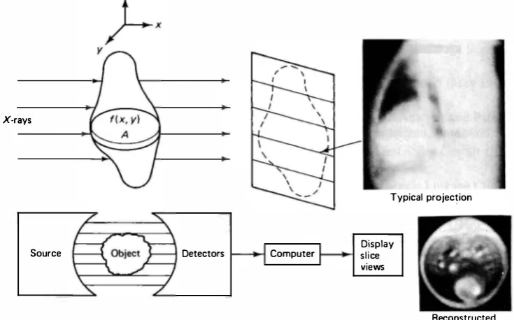
obtained by illuminating an object by penetrating radiation. Figure 10.1 shows a typical method of obtaining projections. Each horizontal line shown in this figure is a one-dimensional projection of a horizontal slice of the object. Each pixel on the projected image represents the total absorption of the X-ray along its path from the source to the detector. By rotating the source-detector assembly around the object, projection views for several different angles can be obtained. The goal of

image reconstruction

is to obtain an image of a cross section of the object from these projections. Imaging systems that generate such slice views are called CT

(computerized tomography)

scanners. Note that in obtaining the projections, we lose resolution along the path of the X-rays. CT restores this resolution by using information from multiple projections. Therefore, image reconstruction from pro­ jections can also be viewed as a special case of image restoration.

Transmission Tomography

For X-ray CT scanners, a simple model of the detected image is obtained as follows. Let

f (x, y)

denote the absorption coefficient of the object at a point

(x, y)

in a slice at some fixed value of

z

(Fig. 10. 1). Assuming the illumination to consist of an infinitely thin parallel beam of X-rays, the intensity of the detected beam is given by

I = lo exp

[

-

{t(x, y) du ]

(10.1)

z

X-rays

Typical projection

Source Detectors Computer slice Display views

Figure 10.1 An X-ray CT scanning system.

Reconstructed cross-section

where /0 _{is the intensity of the incident beam,} L _{is the path of the ray, and} u _{is the} distance along L (Fig. 10.2). Defining the observed signal as

g = In

(�)

(10.2)

we obtain the linear transformation

g

�

g(s, 0) =

J

L

f(x, y) du, -oo < s < oo, O :s 0 < 1T (10.3) where (s, 0) represent the coordinates of the X-ray relative to the object. The image

reconstruction problem is to determine f(x, y) from g(s, 0). In practice we can only estimate f(x, y) because only a finite number of views of g(s, 0) are available. The preceding imaging technique is called transmission tomography because the trans­ mission characteristics of the object are being imaged. Figure 10.1 also shows an X-ray CT scan of a dog's thorax, that is, a cross-section slice, reconstructed from

120 such projections. X-ray CT scanners are used in medical imaging and non­

destructive testing of mechanical objects.

Reflection Tomography

There are other situations where the detected image is related to the object by a transformation equivalent to (10.3). For example, in radar imaging we often obtain

g(s, 0) s

Figure 10.2 Projection imaging geometry in CT scanning.

a projection of the reflectivity of the object. This is called reflection tomography. For instance, in the FLR imaging geometry of Figure 8.7a, suppose the radar pulse width is infinitesimal (ideally) and the radar altitude (h) is large compared to the minor axis of the antenna half-power ellipse. Then the radar return at ground range

r and scan angle <!> can be approximated by (10.3), where f(x, y) represents the ground reflectivity and L is the straight line parallel to the minor axis of the ellipse and passing through the center point of the shaded area. Other examples are found in spot mode synthetic aperture and CHIRP-doppler radar imaging [10, 36).

Emission Tomography

Another form of imaging based on the use of projections is emission tomography, for example, positron emission tomography (PET), where the emissive properties of isotopes planted within an object are imaged. Medical emission tomography ex­ ploits the fact that certain chemical compounds containing radioactive nuclei have a tendency to affix themselves to specific areas of the body, such as bone, blood, tumors, and the like. The gamma rays emitted by the decay of the isotopes are detected, from which the location of the chemical and the associated tissue within the body can be determined. In PET, the radioactive nuclei used are such that positrons (positive electrons) are emitted during decay. Near the source of emis­ sion, the positrons combine with an electron to emit two gamma rays in nearly opposite directions. Upon detection of these two rays, a measurement representing the line integral of the absorption distribution along each path is obtained.

Magnetic Resonance Imaging

Another important situation where the image reconstruction problem arises is in magnetic resonance imaging (MRI). t Being noninvasive, it is becoming increasingly attractive in medical imaging for measuring (most commonly) the density of protons (that is, hydrogen nuclei) in tissue. This imaging technique is based on the funda­ mental property that protons (and all other nuclei that have an odd number of protons or neutrons) possess a magnetic moment and spin. When placed in a mag­ netic field, the proton precesses about the magnetic field in a manner analogous to a top spinning about the earth's gravitational field. Initially the protons are aligned either parallel or antiparallel to the magnetic field. When an RF signal having an appropriate strength and frequency is applied to the object, the protons absorb energy, and more of them switch to the antiparallel state. When the applied RF signal is removed, the absorbed energy is reemitted and is detected by an RF receiver. The proton density and environment can be determined from the charac­ teristics of this detected signal. By controlling the applied RF signal and the sur­ rounding magnetic field, these events can be made to occur along only one line within the object. The detected signal is then a function of the line integral of the MRI signal in the object. In fact, it can be shown that the detected signal is the Fourier transform of the projection at a given angle [8, 9].

Projection-based Image Processing

In the foregoing CT problems, the projection-space coordinates (s, 0) arise nat­ urally because of the data gathering mechanics. This coordinate system plays an important role in many other image processing applications unrelated to CT. For example, the Hough transform, useful for detection of straight-line segments of polygonal shapes (see Section 9.5), is a representation of a straight line in the projection space. Also, two-dimensional linear shift invariant filters can be realized by a set of decoupled one-dimensional filters by working in the projection space. Other applications where projections are useful are in image segmentation (see Example 9.8), geometrical analysis of objects [11] and in image processing applica­ tions requiring transformations between polar and rectangular coordinates.

We are now ready to discuss the Radon transform, which provides the mathe­ matical framework necessary for going back and forth between the spatial coor­ dinates (x, y) and the projection-space coordinates (s, 0).

1 0.2 THE RADON TRANSFORM [12, 13]

Definition

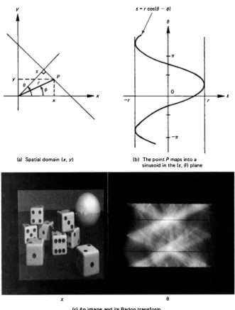
The Radon transform of a function f(x, y ), denoted as g (s, 0), _{is defined as its line} integral along a line inclined at an angle 0 _{from the y-axis and at a distance} s _from

t Also called nuclear magnetic resonance (NMR) imaging. To emphasize its noninvasive features, the word nuclear is being dropped by manufacturers of such imaging systems to avoid confusion with nuclear reactions associated with nuclear energy and radioactivity.

the origin (Fig. 10.2). Mathematically, it is written as

g(s, e)

�

rAt =

Jr

t(x, y)8(x cos e + y sin e - s) dx dy,

-oo < s < oo, 0 $ 0 < 1T (10.4) The symbol rA , denoting the Radon transform operator, is also called the projection

operator. The function g(s, 0), the Radon transform of f(x, y), is the one-dimen­

The quantity g (s, 0) is also called a ray-sum, since it represents the summation of

f(x, y) along a ray at a distance s and at an angle 0. is a sinusoid as shown in Fig. 10.3b. Recall from section 9.5 that the coordinate pair (s, 0) is also the Hough transform of the straight line in Fig. 10.3a.

Example 10.1

Consider a plane wave, f(x, y) = exp[j27T(4x + 3y)]. Then its projection function is

g(s, 0) =

f.,

exp[j87T(s cos 0 - u sin 0)] exp[j67T(s sin 0 + u cos 0)] du

= exp[j27Ts(4 cos 0 + 3 sin 0)]

f.,

exp[-j27Tu(4 sin 0 - 3 cos 0)] du = exp[j27TS (4 COS 0 + 3 sin 0))8( 4 sin 0 - 3 COS 0) = a)ejlO-rrs 8(0 - <j>) where <!> = tan-1a). Here we have used the identity

8[f(0)J ""

�

- 0k)

wheref'(0)

�

df(0)/d0 and 0h k = 1, 2, . . . , are the roots of/(0).

(10.9)

y s = r cos(ll - If>)

y

x s

-r r

(a) Spatial domain (x, y) (b) The point P maps into a

Notation

sinusoid in the (s, 8) plane

x 0

(c) An image and its Radon transform

Figure 10.3 Spatial and Radon transform domains.

In order to avoid confusion between functions defined in different coordinates, we adopt the following notation. Let II be the space of functions defined on JR.2, where

JR denotes the real line. The two-dimensional Fourier transform pair for a function

f(x, y) E '// is denoted by the relation .7z

f(x, y) �-� F(b , b) (10. 10)

In polar coordinates we write

Pp (E, 0) = F(E cos 0 , E sin 0) The inner product in 'lt is defined as

11/11: � (f,f )a

(10.11)

(10.12) Let Vbe the space of functions defined on R x [O, ir]. The one-dimensional Fourier transform of a function g (s, 0) E V is defined with respect to the variable s and is

For simplicity we will generally consider 'it and V to be spaces of real functions. The notation

g = _9lf (10.15)

will be used to denote the Radon transform of f(x, y), where it will be understood that / E 'lt,g E V.

Properties of the Radon Transform

The Radon transform is linear and has several useful properties (Table 10.1), which can be summarized as follows. The projections g(s, 0) are space-limited in s if the object f (

x,

y) is space-limited in (x, y ), and are periodic in 0 with period 2ir. A translation of f(x, y) results in the shift of g(s, 0) by a distance equal to the

pro-TABLE 10.1 Properties of the Radon Transform

438

- 1 .0 -0.8 -0.6 -0.4 -0.2 0.0

-+- X

(a)

(b)

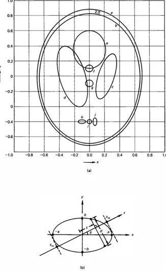
0.2 0.4 0.6 0.8

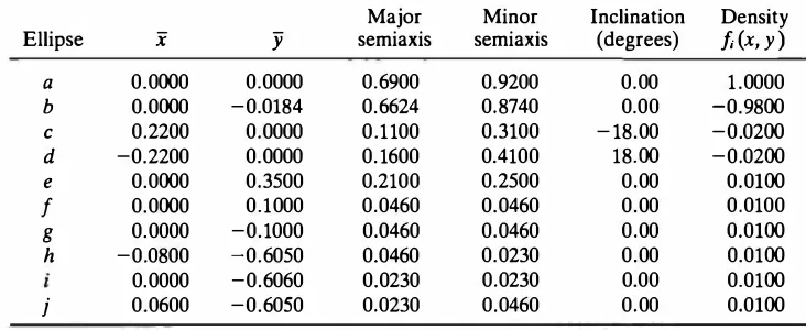
Figure 10.4 (a) Head phantom model; (b) constant-density ellipise, f(x, y) = fo for

(x2/a2) + (y2!b2) :s l .

1 .0

TABLE 10.2 Head Phantom Components; (x, y) are the coordinates of the center of the ellipse. The densities indicated are relative to the density of water [ 1 8] .

Major Minor Inclination Density

Ellipse x _y semiaxis semi axis (degrees) _f; (x, y ) object by an angle

00

causes a translation of its Radon transform in the variable

0.

A scaling of the

(x, y)

coordinates of

f(x, y)

results in scaling of the s coordinate together with an amplitude scaling of

g(s,

0). Finally, the total mass of a distribution

f(x, y)

is preserved by

g(s, 0)

for all

0.

Example 10.2 Computer generation of projections of a phantom

In the development and evaluation of reconstruction algorithms, it is useful to simulate projection data corresponding to an idealized object. Figure 10.4a shows an object composed of ellipses, which is intended to model the human head [18, 21]. Table 10.2 gives the parameters of the component ellipses. For the ellipse shown in Fig. 10.4b, the projection at an angle e is given by

!

2ab -s2 _{I I <} S -Sm

0, lsl > sm

where s;,, = a2 cos2 0 + b2 sin2 0. Using the superposition, translation, and rotation properties of the Radon transform, the projection function for the object of Fig. 10.4a can be calculated (see Fig. 10. 13a).

10.3 THE BACK-PROJECTION OPERATOR

Definition

The quantity b (x, y) is called the back projection of g (s, 0). In polar coordinates it can be written as

b (x, y) = bp (r, <!>) =

r

g(r cos(0 - <J>), 0) d0

0 (10.17)

Back projection represents the accumulation of the ray-sums of all of the rays that pass through the point (x, y) or (r, <!>). For example, if

g(s, 0) = g1 (s)8(0 - 01) + g1 (s )8(0 - 02) that is, if there are only two projections, then (see Fig. 10.5)

bP (r, <!>) = g1 (s1) + g1 (s2)

where s1 = r cos(01 -<!> ), s2 = r cos(02 - <!> ). In general, for a fixed point (x, y) or

(r, <!>), the value of back projection 9Jg is evaluated by integrating g(s, 0) over 0 for all lines that pass through that point. In view of (10.8) and (10.17), the back­ projection at (r, <!>) is also the integration of g(s, 0) along the sinusoid s = r cos(0 -<!>) in the (s, 0) plane (Fig. 10.3b ).

Remarks

The back-projection operator 91 maps a function of (s, 0) coordinates into a func­ tion of spatial coordinates (x, y) or (r, <!> ).

The back-projection b (x, y) at any pixel (x, y) requires projections from all directions. This is evident from (10.16).

440

92 lsl

I I

I I I I I I

' I ' , I

Figure 10.S Back-projection of g, (s)

and g2 (s) at (r, <I>).

It can be shown that the back-projected Radon transform j(x, y)

�

aJg = aJ 91,f

is an image of f(x, y) blurred by the PSF 1/(x2 + y2)112, that is,

f

(x, y) = f(x, y) ® (x2 + y2)-112

(10.18)

(10.19) where ® denotes the two-dimensional convolution in the Cartesian coordinates. In polar coordinates

(10.20) where ® now denotes the convolution expressed in polar coordinates (Problem

10.6). Thus, the operator aJ is not the inverse of 91, . In fact, Y3 is the adjoint of Yr

[Problem 10.7]. Suppose the object f(x, y) and its projections g(s, 0), for all 0 , are discretized and mapped into vectors f and g _{and are related by a matrix trans­} formation g = Rf. The matrix R then is a finite difference approximation of the operator 91, . The matrix RT would represent the approximation of the back­ projection operator aJ .

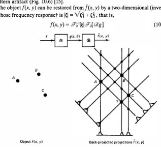
The operation

J

= aJ[ 91,f] gives the summation algorithm (Fig. 10.6). For a set of isolated small objects with a small number of projections, this method gives a star pattern artifact (Fig. 10.6) (15].

The objectf(x, y) can be restored from f(x, y) by a two-dimensional (inverse) filter whose frequency responset is l�I = _�� + �� , that is,

8

• f

c

•

Object f(x, y) _{Back-projected projections f(} x, y)

Figure 10.6 Summation algorithm for image reconstruction, J � .'ii g.

t Note that the Fourier transform of (.t2 + y2r112 is W + m-112•

Sec. 1 0.3 The Back-Projection Operator

(10.21)

TABLE 1 0.3 Filter Functions for Convolution/Filter Back-Projection Algorithms, d

�

1/2 � o

Discrete impulse

Frequency response Impulse response response

Filter _H(�) _h(s) h(m) � dh (md)

where :72 denotes the two-dimensional Fourier transform operator. In practice the filter l�I is replaced by a physically realizable approximation (see Table 10.3). This method [16] is appealing because the filtering operations can be implemented approximately via the FFT. However, it has two major difficulties. First, the Fourier domain computation of l�IF;,(�, 0) gives F(O, 0) = 0, which yields the total density fff(x, y) dx dy = 0. Second, since the support of YJg _{is unbounded, f (x, y) has to be} computed over a region much larger than the region of support off (x, y ). A better algorithm, which follows from the projection theorem discussed next, reverses the order of filtering and back-projection operations and is more attractive for practical implementations.

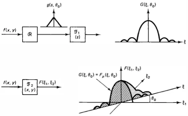
10.4 THE PROJECTION THEOREM [5-7, 12, 13]

There is a fundamental relationship between the two-dimensional Fourier trans­ form of a function and the one-dimensional Fourier transform of its Radon trans­ form. This relationship provides the theoretical basis for several image recon­ struction algorithms. The result is summarized by the following theorem.

Projection Theorem. The one-dimensional Fourier transform with respect

to s _{of the projection} g (s, 0) _{is equal to the central slice, at angle} 0, _{of the two­} dimensional Fourier transform of the object f(x, y), that is, if

g (s, 0) _{G (£,} 0)

then,

G (£, 0) = _F;,(£, 0)

�

_{F(£ cos} 0, _{£ sin} 0) (10.22)

Figure 10.7 shows the meaning of this result. This theorem is also called the

projection-slice theorem.

Proof.

Using (10.6) in the definition of G (I;, e), we can write G (l;, e) �

f,,g(s,

e)e-i2ir� ds

(10.23) =

Jft(s

cos e - u sin e ,

s

sin e + u cos e)e -i2irE-< ds du

Performing the coordinate transformation from

(s,

u) to (x, y), [see (10.5)], this becomes

G (l;, e) =

Jf t

(x,y_{) exp[-j2ir(x l; cas e + y l; sin e)] dx dy}

= F(I; cos e, I; sin e) which proves (10.22).

Remarks

From the symmetry property of Table 10. 1 , we find that the Fourier transform slice also satisfies a similar property

G (-1;, e + ir) = G (I;, e) (10.24)

Iff(x, y) is bandlimited, then so are the projections. This follows immediately from the projection theorem.

An important consequence of the projection theorem is the following result.

f(x, _vl

f(x, y)

Figure 10.7 The projection theorem, G (�, 0) = F,, (�, 0).

Convolution-Projection Theorem. The Radon transform of the two-dimen­ implementation of two-dimensional linear filters by one-dimensional filters. (See Fig. 10.9 and the accompanying discussion in Section 10.5.)

Example 10.3

We will use the projection theorem to obtain the g (s, 0) of Example

10.1.

The

two-dimensional Fourier transform of f(x, y) _{is F( �} i , � 2) = 8( � 1 - 4)8( � 2 - 3) = 8(� cos 0 - 4)8(� sin 0 - 3). From (10.22) this gives G(�, 0) = 8(� cos 0 - 4) 8( � sin 0 - 3). Taking the one-dimensional inverse Fourier transform with respect to � and using the identity (10.9), we get the desired result

g (s, 0) =

r

_{x 8(� cos 0 - 4)8(� sin 0 - 3)ej2T<S�d�}

(

1

) (

j87TS

)

.

= _{lcos 0I} exp cos0 8(4 tan 0 - 3) = G)e110"'s8(0 - <j>)

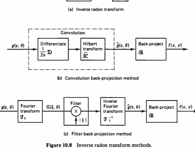
1 0.5 THE INVERSE RADON TRANSFORM [6, _{12, 13, 17]}

The image reconstruction problem defined in Section 10. 1 is theoretically equiv­ alent to finding the inverse Radon transform of g (s, 6). The projection theorem is useful in obtaining this inverse. The result is summarized by the following theorem.

Inverse Radon Transform Theorem. Given g(s, 6) � Yrf, - x < s < oo,

Proof. The inverse Fourier transform

f(x, y) =

fr

F(s " s2) exp[j21T(S , x + by) di; I ds 2

when written in polar coordinates in the frequency plane, gives

Allowing � to be negative and 0 :::; 0 < 11', we can change the limits of integration and use (10.22) to obtain (show!)

f(x, y) =

f' f.,

l�IF;,(�, 0)exp[j211'�(x cos 0 + y sin 0)] d� d0

=

f'

{

f

.,l�IG (�, 0) exp[j211'�(x cos 0 + y sin 0)] d�

}

de (10.29)

=

r

g (x cos 0 + y sin 0, 0) de 0

where

Writing l�IG as �Gsgn(�) and applying the convolution theorem, we obtain g (s, 0) = [ .7[1{�G (�, 0)}] ® [ .7[1{sgn(�)}]

=

[ ��

_{(s, 0)}

]

®

c�� )

=

(-1z) J"'

[

ag (t, e)

J

-1 dt

211' _ ,, at s -t

(10.30)

(10.31)

where (1/j21r)[ag (s, 0)/as] and (- 1/j211's) are the Fourier inverses of �G (�, 0) and sgn(�), respectively. Combining (10.29) and (10.31), we obtain the desired result of (10.26). Equation (10.27) is arrived at by the change of coordinates x = r cos <I> and

y = r sin <I>·

Remarks

The inverse Radon transform is obtained in two steps (Fig. 10.8a). First, each projection g (s, 0) is filtered by a one-dimensional filter whose frequency response is \�\. The result, g (s, 0), is then back-projected to yieldf(x, y). The filtering operation can be performed either in the s domain or in the � domain. This process yields two different methods of finding ur -1, which are discussed shortly.

The integrands in (10.26), (10.27), and (10.31) have singularities. Therefore, the Cauchy principal value should be taken (via contour integration) in evaluating the integrals.

Definition. The Hilbert transform of a function <l>(t) is defined as

ljl(s)

�

.91<1>

�

<f>(s) ®

(

_!__1l'S

)

=

(.!.) J'°

<f>(t) dt

11' -oo S

-

t (10.32)

The symbol .sf-represents the Hilbert transform operator. From this definition it follows that g (s, 0) is the Hilbert transform of (11211')ag (s, 0)/as for each 0.

Because the back-projection operation is required for finding ur -1 , the recon­ structed image pixel at (x, y) requires projections from all directions.

g(s, Ill 1-D filter g(s, II)

Figure 10.8 Inverse radon transform methods.

Convolution Back-Projection Method

Defining a derivative operator as

The inverse Radon transform can be written as

f(x, y) = (l/27r)W _!k·0g

(10.33)

(10.34)

Thus the inverse Radon transform operator is VP -1 = (1/27r) £8 -�''"0 . This means

,q-1 can also be implemented by convolving the differentiated projections with

1/27rs and back-projecting the result (Figure 10.8b).

Filter Back-Projection Method

From (10.29) and (10.30), we can also write f(x, y) = W Sfg

where Sf"is a one-dimensional filter whose frequency response is l�I, that is,

g

�

_srg

�

f.,

_{l�IG(�. e)ei2"�} ds

= _{.711 {l�I[ .71} g]}

(10.35)

(10.36)

This gives

(10.37) which can be implemented by filtering the projections in the Fourier domain and back-projecting the inverse Fourier transform of the result (Fig. IO.Sc).

Example 10.4

We will find the inverse Radon transform of g(s, 0)

= G)ei10"s

8(0 - <!>).

Convolution back-projection method.

Using ag/as = j2

'Trei10"

s8(0 -ti>) in (10.26)

(

jZ'Tr

)

l"f� .

f(X,

y)

=

-2'Tr 2

0 -�

eJIO"s (X

COS 0 + Y Sin 0 - st1 8(0 - tj>)

d

0 ds

= (�) J� ei10"s[s -(x

cos <I> +

y

sin <I> )f

1

ds

]'Tr -�

Since the Fourier inverse of

l/(�

-a) is j'Trei2"a'sgn(t), the preceding integral becomes

f (x,

y) = exp[j2'Tr(x cos ti> + y sin ti> )t] sgn(t)I, � s

=

exp[j

lO'Tr(x

cos ti> + y sin <I>)

J.

Filter back-projection method.

G(�, 0) = G)8(� - 5)8(0 -ti>)

::? t (s, 0) =

G)

f�

1�18(� - 5)8(0 -ti>) exp(j2'Trs�) d�

= ei10"s

8(0 - <1>)

=?f(x,y)=

f

exp[j

lO

'Tr(

x

cos 0 + y sin 0)]8(0 - <l>) d0

=

exp[j

lO'Tr(x

cos <I> + y sin <I>)]

For <I> = tan1

a),f(x, y)

will be the same as in Example 10.1.

Two-Dimensional Filtering via the Radon Transform

A useful application of the convolution-projection theorem is in the implementa­ tion of two-dimensional filters. Let A (� 1 , b) represent the frequency response of a two-dimensional filter. Referring to Fig. 10.9 and eq. (10.25), this filter can be implemented by first filtering for each 6, the one-dimensional projection g(s, 6) by

f(x, y) 2·D filter f(x, y) f(x, y) g(s, 0) 1-D filters q(s, O)

A!�, . �zl _Ap!t 01

Domain

f(x, y) 1-D filters g(s, Ol

I � I Ap(t Ol

Figure 10.9 Generalized filter back projection algorithm for two-dimensional fil­ ter implementation.

Sec. 1 0.5 The Inverse Radon Transform

f(x, y)

f(x, y)

a one-dimensional filter whose frequency response is AP (�, 0) and then taking the inverse Radon transform of the result. Using the representation of �-1 in Fig. 10.8a, we obtain a generalized filter-back-projection algorithm, where the filter now becomes l�IAP (�, 0). Hence, the two-dimensional filter A (� _{1 ,} �1) can be imple­ mented as

a (x, y) © f(x, y) = q; SfBg (10.38)

wh�re %e represents a one-dimensional filter with frequency response Ap (�, 0)

�

l�IAp (�, 0).

1 0.6 CONVOLUTION/FILTER BACK-PROJECTION ALGORITHMS : DIGITAL IMPLEMENTATION [18-21]

The foregoing results are useful for developing practical image reconstruction algorithms. We now discuss various considerations for digital implementation of these algorithms.

Sampling Considerations

In practice, the projections are available only on a finite grid, that is, we have available

gn (m)

�

g(sm, 0n)

�

[ _{9cf](sm ,} 0n),

(10.39)

where, typically, Sm = md, an = n!l., /:l. = TrlN. Thus we have N projections taken at equally spaced angles, each sampled uniformly with sampling interval d. If � 0 is the highest spatial frequency of interest in the given object, then d should not exceed the corresponding Nyquist interval, that is, d :::::; 1/2� 0 • If the object is space limited, that is, fp (r, <!>) = 0, lrl > D/2, _then D =Md_{, and the number of samples should} satisfy

(10.40)

Choice of Filters

The filter function l�I required for the inverse Radon transform emphasizes the high-spatial frequencies. Since most practical images have a low SNR at high fre­ quencies, the use of this filter results in noise amplification. To limit the unbounded nature of the frequency response, a bandlimited filter, called the Ram-Lak filter

[19)

(10.41) has been proposed. In practice, most objects are space-limited and a bandlimiting filter with a sharp cutoff frequency � 0 is not very suitable, especially in the presence

of noise. A small value of � 0 gives poor resolution and a very large value leads to noise amplification. A generalization of (10.41) is the class of filters

H(�) = l�IW(�) (10.42)

Here W(�) is a bandlimiting window function that is chosen to give a more­ moderate high-frequency resppnse in order to achieve a better trade-off between the filter bandwidth (that is, high-frequency response) and noise suppression. Table 10.3 lists several commonly used filters. Figure 10.10 shows the frequency and

Frequency response HW Impulse response h (s)

0.3

Figure IO. IO Reconstruction filters. Left column: Frequency response; right

col-umn: Impulse response; dotted lines show linearly interpolated response.

i.lm)

Discrete

g.(m)

_Linear

9.<si

Discrete "" f( x, y) convolution _{interpolation} back-projection

A

ffi N

h(m)

(a) Convolution back-projection algorithm: Digital implementation ;

f-gn(ml0-j

(b) Filter back-projection algorithm: Digital implementation.

Figure 10. 11 Implementation of convolution/filter back projection algorithms.

the impulse responses of these filters for d = 1. Since these functions are real and even, the impulse responses are displayed on the positive real line only. For low levels of observation noise, the Shepp-Logan filter is preferred over the Ram-Lak filter. The generalized low-pass Hamming window, with the value of a optimized for the noise level, is used when the noise is significant. In the presence of noise a better approach is to use the optimum mean square reconstruction filter also called the stochastic filter, (see Section 10.8).

Once the filter has been selected, a practical reconstruction algorithm has two major steps:

1. For each 0, filter the projections g(s, 0) by a one-dimensional filter whose frequency response is H ( �) or impulse response is h (s ).

2. Back-project the filtered projections, g(s, 0).

Depending on the implementation method of the filter, we obtain two distinct algorithms (Fig. 10.11). In both cases the back-projection integral [see eq. (10. 17)] is implemented by a suitable finite-difference approximation. The steps required in the two algorithms are summarized next.

Convolution Back-Projection Algorithm

The filtering operation is implemented by a direct convolution in the s do­ main. The steps involved in the digital implementation are as follows:

1. Perform the following discrete convolution as an approximate realization of sampled values of the filtered projections, that is,

M/2- 1 _{-M M}

g(md, nil) = gn(m) � L 8n(k)k (m - k), - :5 m :5- - l _{k = -M/2 2 2} (10.44)

where h(m) � dh(md) is obtained by sampling and scaling h(s). Table 10.3 lists h (m) for the various filters. The preceding convolution can be imple­ mented either directly or via the FFT as discussed in Section 5.4.

2. Linearly interpolate gn(m) to obtain a piecewise continuous approximation of

g(s, nil) as

g(s, nil) = frn(m) +

(�

- m

)

[gn(m + 1) - gn(m)],

(10.45) md :ss < (m + l)d

3. Approximate the back-projection integral by the following operation to give N- 1

f(x, y) =f(x, y) � {l]Ng � Ll L g(x cosntl + y sinntl, ntl) (10.46)

n = O

where {lJ _N is called the discrete back-projection operator. Because of the back­ projection operation, it is necessary to interpolate the filtered projections

8n(m). This is required even if the reconstructed image is evaluated on a sampled grid. For example, to evaluate

N-1

f(i Llx.j fly) = fl L g (iflx cos n fl + j fly sin n fl, nil) (10.47) n=O

on a grid with spacing (Ax, Ay), i, j = 0, ± _1, ±2, _{. . . , we still need to evaluate}

g(s, nA) at locations in between the points md, m

=

-M/2, . . . ,M/2 - 1. Al­ though higher-order interpolation via the Lagrange functions (see Chapter 4) is possible, the linear interpolation of (10.45) has been found to give a good trade-off between resolution and smoothing [18]. A zero-order hold is some­ times used to speed up the back-projection operation for hardware imple­ mentation.

Filter Back-Projection Algorithm

In Fig. 10.llb, the filtering operation is performed in the frequency domain accord­ ing to the equation

g(s, 0)

=

.9""!1[G (�, 0)H(�)] (10.48) Given H(�), the filter frequency response, this filter is implemented approximately by using a sampled approximation of G (�, 0) and substituting a suitable FFT for the

inverse Fourier transform. The algorithm is shown in Fig. 10. llb, which is a one­ dimensional equivalent of the algorithm discussed in Section 8.3 (Fig. 8.13b). The steps of this algorithm are given next:

1. Extend the sequence gn (m ), -M 12 :s: m :s: (M /2) - 1 by padding zeros and

periodic repetition to obtain the sequence gn (m)0 0 :s: m :s: K - 1 . Take its

FFT to obtain G n ( k ), 0 :s: k :s: K - 1 . The choice of K determines the sampling resolution in the frequency domain. Typically K = 2M if M is large; for exam­ ple, K = 512 if M = 256.

2. Sample H(�) to obtain

H

(k)

�

H(kb.�),

H

(K - k)

�

H*(k), 0 :s: k < K/2,

where * denotes the complex conjugate.

3. Multiply the sequences Gn (k) and

H

(k), 0 :s: k :s: K - 1 , and take the inverse

FFT _{of the product. A periodic extension of the result gives 8n} (m), -K/2 :s: m :s: (K/2) - 1 . The reconstructed image is obtained via (10.45) and

(10.46) as before.

Example 10.5

Figure 10.12b shows a typical projection of an object digitized on a 128 x 128 grid (Fig. 10.12a). Reconstructions obtained from 90 such projections, each with 256 samples per line, using the convolution back-projection algorithm with Ram-Lak and Shepp-Logan filters, are shown in Fig. 10.12c and d, respectively. Intensity plots of the object and its reconstructions along a horizontal line through its center are shown in Fig. 10.12f through h. The two reconstructions are almost identical in this (noiseless) case. The background noise that appears is due to the high-frequency response of the recon­ struction filter and is typical of inverse (or pseudoinverse) filtering. The stochastic filter outputs shown in Fig. 10.12e and i show an improvement over this result. This filter is discussed in Section 10.8.

Reconstruction Using a Parallel Pipeline Processor

Recently, a powerful hardware architecture has been developed [11] that en­ ables the high speed computation of digital approximations to the Radon transform and the back-projection operators. This allows the rapid implementation of convolution/filter back-projection algorithms as well as a large number of other image processing operations in the Radon space. Figure 10.13 shows some results of reconstruction using this processor architecture.

10.7 RADON TRANSFORM OF RANDOM FIELDS _{[22, 23]}

So far we have considered /(x, y) to be a deterministic function. In many problems, such as data compression and filtering of noise, it is useful to consider the input f(x, y) to be a random field. Therefore, it becomes necessary to study the properties

of the Radon transform of random fields, that is, projections of random fields.

A Unitary Transform �

Radon transform theory for random fields can be understood more easily by consid­ ering the operator

+

•

•

+

•

+ _• + + _•

+ +

+

(a) Original object

•

• • •

•

0

•

(c) Ram-Lak filter

(e) Stochastic filter

g(s, 0)

I

40

30

20

1 0

-10

- 1 28 -g6 -64 -32 0 32 64

- s

(bl A typical projection

•

• • _•

•

•

0

•

(d) Shepp-Logan filter

Figure 10.12 Image reconstruction example.

96 1 28

3 3

2 2

0 0

-1 - 1

-64 -48 -32 - 1 6 0 1 6 32 48 64 -64 -48 -32 - 1 6 0 1 6 32 48 64

(f) Object l ine

3

2

0

- 1

3

2

0

- 1

(g) Reconstruction via RAM-LAK filter

-64 -48 -32 -16 0 16 32 48 64 -64 -48 -32 - 1 6 0 16 32 48 64

(h) Reconstruction via Shepp-Logan filter

Figure 10.12 Cont'd

(i) Reconstruction via stochastic filter. Also see Example 1 0.6

(10.49)

where 51[112 represents a one-dimensional filter whose frequency response is lsl112• The operation

(10.50)

is equivalent to filtering the projections by 9'("112 (Fig. 10.14). This operation can also be realized by a two-dimensional filter with frequency response (s� + s�)114 followed by the Radon transform.

Theorem 10.1. Let a + denote the adjoint operation of 9c . The operator 9c

is unitary, that is,

a _-1 = a + = aJ :7(-112 (10.51)

This means the inverse of a is equal to its adjoint and the a transform preserves energy, that is,

(a) Original phantom image

abcdefg

l1ijl{lmn

opqrstu

vw_xyz

.,

(b) reconstruction via convolution back-projection,

l1ijlclmn

opqrst11

vwxyz

(c) original binary image (d) reconstruction using fully constrained ART

algorithm

Figure 10.13 Reconstruction examples using parallel pipeline processor.

ff

1t(x, y)l2dxdy =

r r

jg (s, 0)12dsd0

- � 0 -�

(10.52)

This theorem is useful for developing the properties of the Radon transform for random fields. For proofs of this and the following theorems, see Problem 10.13.

f

Figure 10.14 The .Cf-transform.

Radon Transform Properties for Random Fields

Definitions. Let f(x, y) be a stationary random field with power spectrum

density S(£ i. £2) and autocorrelation function r(Ti.T2). Then S(£ i. £2) and r(Ti,T2) form a two-dimensional Fourier transform pair. Let SP (£, 6) denote the polar­ coordinate representation of S(£ i, £2), that is,

SP (�, 6) � S(� cos 6, � sin 6) (10.53) Also, let rP (s, 6) be the one-dimensional inverse Fourier transform of SP (£, 6), that is,

(10.54) Applying the projection theorem to the two-dimensional function r(Ti. T2), we ob­ serve the relation

rP (s, 6) = U?r (10.55)

Theorem 10.2. The operator ?f is a whitening transform in 6 for stationary

random fields, and the autocorrelation function of g (s, 6) is given by

where

r88 (s, 6; s ', 6') � E [g (s, 6)g (s ', 6')] = r8 (s - s ', 6)8(6 - 6') (10.56a)

r8 (s, 6) = rP (s, 6) (10.56b)

This means the random field g (s, 6) defined via (10.50) is stationary in s and uncorrelated in 6. Since g (s, 6) can be obtained by passing g (s, 6) through .W-112, which is independent of 6, g(s, 6) itself must be also uncorrelated in 6. Thus, the Radon transform is also a whitening transform in 6 for stationary random fields and the autocorrelation function of g (s, 6) must be of the form

rgg (s, 6;s '; 6') � E[g(s, 6)g(s ', 6')] = rg(s - s ', 6)8(6 - 6') (10.57) where rg (s, 6) is yet to be specified. Now, for any given 6, we define the power spectrum density of g (s, 6) as the one-dimensional Fourier transform of its auto­ correlation function with respect to s, that is,

(10.58)

From Fig. 10. 14 we can write

(10.59)

These results lead to the following useful theorem.

Projection Theorem for Random Fields

Theorem 10.3. The one-dimensional power spectrum density S8 (s, 0) of the 9l

transform of a stationary random field f(x, y) is the central slice at angle 0 of its two-dimensional power spectrum density S(s 1 , s2), that is,

(10.60)

This theorem is noteworthy because it states that the central slice of the two­ dimensional power spectrum density S ( s 1 , s 2) is equal to the one-dimensional power spectrum of g (s, 0) and not of g(s, 0). On the other hand, the projection theorem states that the central slice of a two-dimensional amplitude spectrum den­

sity (that is, the Fourier transform) F ( s 1 , s 2) is equal to the one-dimensional ampli­

tude spectrum density (that is, the Fourier transform) of g(s, 0) and not of g (s, 0). Combining (10.59) and (10.60), we get

(10.61) which gives, formally,

(10.62)

and

(10.63)

Theorem 10.3 is useful for finding the power spectrum density of noise in the reconstructed image due to noise in the observed projections. For example, suppose

v(s, 0) is a zero mean random field, given to be stationary in s and uncorrelated in 0, with

E[v(s, 0)v(s ', 0')] = _{rv (s - s ', 0)8(0 - 0')}

.71

Sv (s, 0) rv (s, 0)

(10.64a) (10.64b) If v(s, 0) represents the additive observation noise in the projections, then the noise component in the reconstructed image will be

TJ(X, y) � aJ _Sf'v = aJ %112 ii = £7l -l ii

where

ii �

�12v. Rewriting (10.65) as

ii = m 'TJ

Sec. 1 0.7 Radon Transform of Random Fields

(10.65)

(10.66)

and applying Theorem 10.3, we can write STJP (�, 0), the power spectrum density of TJ ,

as

(10.67) This means the observation noise power spectrum density is amplified by (�� + �1)112 by the reconstruction process (that is, by 01-1). The power spectrum STI is bounded only if l�IS" (�, 0) remains finite as �� oo. For example, if the random field v(s, 0) is bandlimited, then TJ(X, y) will also be pandlimited and STI will remain bounded.

1 0.8 RECONSTRUCTION FROM BLURRED NOISY PROJECTIONS [22-25)

Measurement Model

In the presence of noise, the reconstruction filters listed in Table 10.3 are not optimal in any sense. Suppose the projections are observed as

w (s, 0) =

f.,

hp (s - s ', 0)g(s ', 0) ds ' + v(s, 0), _(10.68) -00 < s < oo, 0 < 0 ::5 1T

The function hP (s, 0) represents a shift invariant blur (with respect to s), which may occur due to the projectiG>n-gathering instrumentation, and v(s, 0) is additive, zero mean noise independent of f(x, y) and uncorrelated in 0 [see (10.64a)]. The opti­ mum linear mean square reconstruction filter can be determined by applying the Wiener filtering ideas that were discussed in Chapter 8.

The Optimum Mean Square Filter

The optimum linear mean square estimate of f(x, y), denoted by

J

(x, y), can be reconstructed from w (s, 0), by the filter/convolution back-projection algorithm (Problem 10.14)

where

Remarks

g (s, 0) =

f,,

ap (s - s', e)w(s ', e) ds'

/ (x, y) = alg _(10.69)

(10.70)

The foregoing optimum reconstruction filter can be implemented as a generalized filter/convolution back-projection algorithm using the techniques of Section 10.6. A

provision has to be made for the fact that now we have a one-dimensional filter

aP

(s, 0), which can change with 0.

Reconstruction from noisy projections. In the absence of blur we have

hp (s, 0) = o(s) and

w₍s, 0) = g(s, 0) + v(s, 0) The reconstruction filter is then given by

_

!�ISP (�,

0)

AP (�,

0)

_{- [Sp(�,}

₀₎

₊

_{1�1s. (�,}

_0)]

(10.71)

(10.72)

Note that if there is no noise, that is, s.� 0, then

AP(�,

0)�

1

�

1, which is, of course, the filter required for the inverse Radon transform.

Using (10.61) in (10.70) we can write

AP(�,

0) =

l�IAP (�,

0) (10.73)

where

(10.74)

Note that

AP (�,

0)

is the one-dimensional Weiner filter for g (s, 0) given w(s,

0).

This means the overall optimum filter

AP

is the cascade of

l�I,

the filter required for the inverse Radon transform, and a window function

Ay (�,

0), representing the locally optimum filter for each projection. In practice,

AP(�,

0) can be estimated adaptively for each 0 by estimating

Sw (�,

0),

the power spectrum density of the observed projection w(s, 0).

Example 10.6 Reconstruction from noisy projections

Suppose the covariance function of the object is modeled by the isotropic function r(x, y) = a2 + y 2). _{The corresponding power spectrum is then} S (� i. b) =

2imcr 2[a2 ₊ 4ir2 (�; ₊ ��)t3ri _or Sp (�, ₀₎ = 2iraa 2[a2 + 4ir2 er3n. _{Assume there is no}

blur and let r. (s, 0) = a� . Then the frequency response of the optimum reconstruction

filter, henceforth called the stochastic filter, is given by

2iro:cr 2 + l�ld;. ( o:2 + 4ir2 � 2)3!2

l�l2iro:(SNR) _{SNR �} a2

- 2 (1 v

This filter is independent of 0 _{and has a frequency response much like that of a}

band-pass filter (Fig. 10.15a). Figure 10.15b shows the impulse response of the sto­ chastic filter used for reconstruction from noisy projections with a� = _5, a 2 = 0.0102, and a = _{0.266. Results of reconstruction are shown in Fig. 10.15c through i. Com­}

parisons with the Shepp-Logan filter indicate significant improvement results from the use of the stochastic filter. In terms of mean square error, the stochastic filter performs 13.5 dB better than the Shepp-Logan filter in the case of a� = _{5. Even in the noiseless}

case (Fig. 10.12) the stochastic filter designed with a high value of SNR (such as 100), provides a better reconstruction. This is because the stochastic filter tends to moderate the high-frequency components of the noise that arise from errors in computation.

0.70

0.60

0.50

Ap (t B) 0.40

I

0.30 0.20

0.10

1 .0

0.8

0.6

h(s) 0.4

t

0.2 0

-0.2

-0.4 0

460

4

(al A typical frequency response of a stochastic tilter

AP (t Bl = AP (-�. e)

8 1 2 1 6 20

---1- s

(b) I mpulse response of the stochastic filter used

24

Figure 10.15 Reconstruction from noisy projections.

28

Image Reconstruction from Projections 32

30 3

2

20

1 0

0

0 _{- 1}

- 1 0 - 2

- 1 28 -96 -64 -32 0 32 64 96 1 28 -64 -48 -32 - 1 6 0 1 6 32 48 64

(c) Typical noisy projection, a� = 5 (d) Reconstruction via Shepp-Logan filter

3

2

0

- 1

-64 -48 -32 - 1 6 0 1 6 32 48 64

(e) Reconstruction via the stochastic filter

(f) Shepp-Logan filter, a� = 1 ; (g) Stochastic filter, a� = 1 ;

Figure 10. 15 Cont'd

(h) Shepp-Logan filter, er� = 5; (i) Stochastic filter, er� = 5.

Figure 10.15 Cont'd

1 0.9 FOURIER RECONSTRUCTION METHOD [2₆-29]

A conceptually simple method of reconstruction that follows from the projection theorem is to fill the two-dimensional Fourier space by the one-dimensional Fourier transforms of the projections and then take the two-dimensional inverse Fourier transform (Fig. 10. 16a), that is,

Algorithm

f(x, y) = _{.-721 [ c7"1g]} (10.75)

There are three stages of this algorithm (Fig. 10. 16b). First we obtain

Gn (k) = G (kl1E, n fl0), -K/2 :::; k ::5 K/2 - l , 0 ::5 n ::5 N - l , as in Fig. (10.l lb).

Next, the Fourier domain samples available on a polar raster are interpolated to yield estimates on a rectangular raster (see Section 8. 16). In the final stage of the algorithm, the two-dimensional inverse Fourier transform is approximated by a suitable-size inverse FFf. Usually, the size of the inverse FIT is taken to be two to three times that of each dimension of the image. Further, an appropriate window is used before inverse transforming in order to minimize the effects of Fourier domain truncation and sampling.

Although there are many examples of successful implementation of this algorithm [29], it has not been as popular as the convolution back-projection algo­ rithm. The primary reason is that the interpolation from polar to raster grid in the frequency plane is prone to aliasing effects that could yield an inferior reconstructed image.

g(s, 11)

Yn (m)c Gn (k)

G(t lll

F i l l Fourier space

(a) The concept

Interpolate F(kA�1 • /A�2l

from polar to rectangular raster

F(t1 • t2)

Window and/or

pad zeros

0 0 0 0

0 0 0 0

f(x, y)

2-D inverse

F FT

k

0 0 0 0

0 0 0 0

(b) A practical fourier reconstruction algorithm

Figure 10.16 Fourier reconstruction method.

"

f(mAx, nAy)

Reconstruction of Magnetic Resonance Images (Fig. 1 0. 17)

In magnetic resonance imaging there are two distinct scanning modalities, the projection geometry and the Fourier geometry [30]. In the projection geometry mode, the observed signal is G (�, 0), sampled at � = kA�, -K/2 ::s k ::s K/2 - l, 0 = n A0, 0 ::s n ::s N -1, A0 = 'ITIN. Reconstruction from such data necessitates the

availability of an FFf processor, regardless of which algorithm is used. For exam­ ple, the filter back-projection algorithm would require inverse Fourier transform of

Sec. 1 0.9

(a) MRI data; (b) Reconstructed image;

Figure 10.17 Magnetic resonance image reconstruction.

G(�, e)H(�). Alternatively, the Fourier reconstruction algorithm just described is also suitable, especially since an FFf processor is already available.

In the Fourier geometry mode, which is becoming increasingly popular, we directly obtain samples on a rectangular raster in the Fourier domain. The recon­ struction algorithm then simply requires a two-dimensional inverse FFf after win­ dowing and zero-padding the data.

Figure 10. 17a shows a 512 x 128 MRI image acquired in Fourier geometry mode. A 512 x 256 image is reconstructed (Fig. 10. 17b) by a 512 x 256 inverse FFf of the raw data windowed by a two-dimensional Gaussian function and padded by zeros.

1 0. 1 0 FAN-BEAM RECONSTRUCTION

Often the projection data is collected using fan-beams rather than parallel beams (Fig. 10. 18). This is a more practical method because it allows rapid collection of projections C9mpared to parallel beam scanning. Referring to Fig. 10.18b, the source S emits a thin divergent beam of X-rays, and a detector receives the beam after attenuation by the object. The source position is characterized by the angle 13, and each projection ray is represented by the coordinates (CT, 13), -TI/2 :s CT < TI/2, 0 :s 13 < 2TI. The coordinates of the (CT, 13) ray are related to the parallel beam

coordinates (s, e) as (Fig. 10. 18c)

s = R sin CT _(10.76)

e = CT + l3

where R is the distance of the source from the origin of the object. For a space­ limited object with maximum radius D 12, the angle CT lies in the interval [--y, -y], -y � sin-1 (D/2R ). Since a ray in the fan-beam geometry is also some ray in the parallel beam geometry, we can relate their respective projection functions b (CT, 13) and g(s, e) .as available on a uniform grid, we can use the foregoing parallel beam reconstruction algorithms. Another alternative is to derive the divergent beam reconstruction algorithms directly in terms of b ( <r, 13) by using (10. 77) and (10. 78) in the inverse

Radon tran�form formulas. (See Problem 10.16.)

In practice, rebinning seems to be preferred because it is simpler and can be fed into the already developed convolution/filter back-projection algorithms (or

(a) Paral lei beam

(c) Fan beam geometry

(b) Fan beam

Projection ray

Figure 10.18 Projection data acquisition.

Detector

processors). However, there are situations where the data volume is so large that the storage requirements for rebinning assume unmanageable proportions. In such cases the direct divergent beam reconstruction algorithms would be preferable because only one projection, b (cr, 13), would be used at a time, in a manner charac­ teristic of the convolution/filter back-projection algorithms.

1 0. 1 1 ALGEBRAIC METHODS

All the foregoing reconstruction algorithms are based on Radon transform theory and the projection theorem. It is possible to formulate the reconstruction problem as a general image restoration problem solvable by techniques discussed in Chapter 8.

The Reconstruction Problem as a Set of Linear Equations

Suppose f(x, y) is approximated by a finite series

I J

f(x, y) =

J

(x, y) = L L a;,i<f>i.i (x, y)

i = l j = I

where {<f>;.i (x, y)} is a set of basis functions. Then

Sec. 1 0. 1 1

I J I J

g(s ' 0) = �f� = 1, J ·] � 1, J 1, J ·h· ·(s ' 0) i = l j = l i = l j =

I

Algebraic Methods

(10.79)

(10.80)

where h;,i (s, e) is the Radon transform of <!>;.i (x, y), which can be computed in obtained directly from (10. 79).

A particular case of interest is when f(x, y) is digitized on, for instance, an realistic observation equation is of the form

(10.85) where 1l represents noise. The reconstruction problem now is to estimateJfrom�.

Equations (10.84) and (10.85) are now in the framework of Wiener filtering, pseudoinverse, generalized inverse, maximum entropy, and other restoration algo­ rithms considered in Chapter 8. The main advantage of this approach is that the algorithms needed henceforth would be independent of the scanning modality (e.g., paralfel beam versus fan beam). Also, the observation model can easily incorporate a more realistic projection gathering model, which may not approximate well the Radon transform.

The main limitations of the algebraic formulation arise from the large size of the matrix .9C. For example, for a 256 x 256 image with 100 projections each sampled to 512 points, .9'Cbecomes a 51,200 x 65,536 _{matrix. However, .9'Cwill be}

a highly sparse matrix containing only 0 (/) or 0 (J) nonzero entries per row. These nonzero entries correspond to the pixel locations that fall in the path of the ray (sm , en). Restoration algorithms that exploit the sparse structure of .9'Care feasible.

Algebraic Reconstruction Techniques

A subset of iterative reconstruction algorithms have been historically called ART (algebraic reconstruction techniques). These algorithms iteratively solve a' set of P equations

p = 0, . . . , P - 1 (10.86)

where h-� is the pth row of .9C and _{,9' P} is the pth element of,y . The algorithm, originally due to Kaczmarz (30], has iterations that progress cyclically as

J- (k + I) =J(k) _{llh-k + 1 112} h,, k + I ' k = 0, 1, . . . (10.87)

wherif (k + 'l determineif<k + 'l, depending on the constraints imposed on J(see

Table 10.4), J<0> is some initial condition, and,yk and h-k appear cyclically, that is,

(10.88)

Each iteration is such that only one of the P equations (or constraints) is satisfied at a time. For example, from (10.87) we can see

<h-k + 1 ,J- (k+ l)) = (h-k+ l ,J(k))+ [,_9k+ 1 - ) llh.k + 1 112 k + I ' h,,k +

I (10.89)

=,jl k + I

that is, the [(k + 1) modulo P]th constraint is satisfied at (k + l)th iteration. This algorithm is easy to implement since it operates on one projection sample at a time. The operation (h-k + 1 ,J<kl) is equivalent to taking the [(k + 1) modulo P]th pro­

jection sample of the previous estimate. The sparse structure of h-k can easily be exploited to reduce the number of operations at each iteration. The speed of con­ vergence is usually slow, and difficulties arise in deciding when to stop the iter­ ations. Figure 10.13d shows an image reconstructed using the fully constrained ART algorithm in (10.87). The result shown was obtained after five complete passes through the image starting from an all black image.

TABLE 1 0.4 ART Algorithms algorithm converges to the element of L1 with the smallest distance to J (OJ. If L2 � {J l.9ll"= ..9'' .//?::. O} is nonempty,

the algorithm converges to an element of

L2.

If L3 � {J 1.9ll"= ..9'• 0 :5j/:5 l} is non­ empty, the algorithm converges to an element of L3•

1 0.12 THREE-DIMENSIONAL TOMOGRAPHY

If a three-dimensional object is scanned by a parallel beam, as shown in Fig. 10. 1, then the entire three-dimensional object can be reconstructed from a set of two­ dimensional slices (such as the slice A ), each of which can be reconstructed using the foregoing algorithms. Suppose we are given one-dimensional projections of a three-dimensional object f(x, y, z). These projections are obtained by integrating

f(x, y, z) in a plane whose orientation is described by a unit vector a (Fig. 10. 19), that is,

g (s, a₎= [ 92/](s, a)=

IJr

f(x)8(x7 _Q'. -s) dx

(10.90)

=

Jf J"

_{f(x, y, z)8(x} sin 0 cos <!> + y sin 0 sin <!> + z cos 0 -s] dx dy dz

_..,

where x � [x, y, z y, a� [sin 0 cos <j>, sin 6 sin <j>, cos ey. This is also called the

three-dimensional Radon transform of f(x, y, z). The Radon transform theory can

be readily generalized to three or higher dimensions. The following theorems

provide algorithms for reconstruction of/(x, y, z) from the projections g(s, a).

Three-Dimensional Projection Theorem. The one-dimensional Fourier trans­ form of g(s, a) defined as

G (£_,a) �

r.

g (s, a)e -i2"E.s ds _{(10. 91)}

is the central slice F( £a) iri the direction a of the three-dimensional Fourier trans­

form of f(x), that is,

z

x

468

G (£,a) = F(£a) � F(£ sin e cos cj>, £ sin e sin cj> , £ cas e) (10.92)

Figure 10.19 Projection geometry for three-dimensional objects.

g (s , o:I _{1 a2g (s, o:)} #(s, o:) f(x, y, zl

Figure 10.20 Three-dimensional inverse radon transform.

where

F(�1 , �2 , �3) = F(�) �

Jf f

f(x)e-i211<xT�) dx,

Three-Dimensional Inverse Radon Transform Theorem. The inverse of the

three-dimensional Radon transform of (10.90) is given by (Fig. 10.20)

where Proofs and extensions of these theorems may be found in [13).

Three-Dimensional Reconstruction Algorithms

(10.94)

(10.95)

The preceding theorem gives a direct three-dimensional digital reconstruction algo­ rithm. If g (sm, «n) are the sampled values of the projections given for Sm = md, -M 12 s m s M 12 - 1, 0 s n s N - 1, for instance, then we can approximate the

second partial derivative by a three-point digital filter to give

A 1 �- -�

g (sm, «n) = 81T2d2[2g(md, «n) -g(m - ld, «n) -g(m + ld, «n)) (10.96) In order to approximate the back-projection integral by a sum, we have to sample <j> and 0, where (<l>b 0i) define the direction «n . A suitable arrangement for the projection angles ( <l>b 0J is one that gives a uniform distribution of the projections over the surface of a sphere. Note that if 0 and <j> are sampled uniformly, then the projections will have higher concentration near the poles compared to the equator. If 0 is sampled uniformly with ae = 1Tll, we will have 0i = (j + !)ae, j = 0, 1, . . . , J - 1. The density of projections at elevation angles 0i will be proportional to l/sin 0i . Therefore, for uniform distribution of projections, we should increment <!>k in proportion to 1/sin 0i, that is, il<j> = c/sin 0i, <!>k = kil<j>, k = 0, . . . , K -1, where c

is a proportionality constant. Since <!>K must equal 21T, we obtain

-21Tk

- K· _I ' k = 0, 1,

. . . , Ki -l

/ (10.97)

This relation can be used to estimate Ki to the nearest integer value for different 0i .

g(s, cd f(x, y, z)

Figure 10.21 Two-stage reconstruction.

The back-projection integral is approximated as • • /:J.. 211'2 stages of two-dimensional inverse Radon transforms. In the first stage, q, is held constant (by �;,�) and in the second stage, z is held constant (by

f/l;.�<1>)·

Details are given in Problem 10. 17. Compared to the direct method, where an arbitrary section of the object can be reconstructed, the two-stage algorithm necessitates recon­ struction of parallel cross sections of the object. The advantage is that only two­ dimensional reconstruction algorithms are needed.

1 0.13 SUMMARY

In this chapter we have studied the fundamentals and algorithms for reconstruction of objects from their projections. The projection theorem is a fundamental result of Fourier theory, which leads to useful algorithms for inverting the Radon transform. Among the various algorithms discussed here, the convolution back projection is the most widely used. Among the various filters, the stochastic reconstruction filter seems to give the best results, especially for noisy projections. For low levels of noise, the modified Shepp-Logan filter performs equally well.

The Radon transform theory itself is very useful for filtering and representa­ tion of multidimensional signals. Most of the results discussed here can also be extended to multidimensions.

PROBLEMS

10.1 Prove the properties of the Radon transform listed in Table 10. 1.

10.2 Derive the expression for the Radon transform of the ellipse shown in Figure 10.4b.

10.3 Express the Radon transform of an object f _{P (r, <!>) given in polar coordinates.}

10.4 Find the Radon transform of a. exp(-7r(x2 + y2)], 'r/x, y

b. (kx + ly)

J, -%

s x, y s

%

-rrkx -rrly L L

c. cosL cosy, -2sx, y s2

d. cos2-rr(ax + (3y), + y2 s a

Assume the given functions are zero outside the region of support defined.

10.5 Find the impulse response of the following linear systems.

� �

Figure Pl0.5

10.6 In order to prove (10.19), use the definitions of u'3 and !I? to show that

1

(x, y) =

11�

f(x 11 y

')[r

8((x I - x) cos 0 + (y I - y) sin 0) d0

]

dx I dy I

Now using the identity (10.9), prove (10.19). Transform to polar coordinates and prove (10.20).

10.7 Show that the back-projection operator 11J is the adjoint of !I? . This means for any

a (x, y) E ii and b (s, 0) E 'P, show that ( !/?a, b ),, = (a, 1/J b ),, .

10.8 Find the Radon transforms of the functions defined in Problem 10.4 by applying the

projection theorem.

10.9 Apply the projection theorem to the function f(x, y) �fl _(x, y) 0 f2 (x, y) and show

,71[ fh'f] = G1 (�, 0)G2 (�, 0). From this, prove the convolution-projection theorem.

10.10 Using the formulas (10.26) or (10.27) verify the inverse Radon transforms of the results obtained in Problem 10.8.

10.11 If an object is space limited by a circle of diameter D and if � o is the largest spatial frequency of interest in the polar coordinates of the Fourier domain, show the number of projections required to avoid aliasing effects due to angular sampling in the trans­ form domain must be N > -rr D � 0 •

10.12* Compute the frequency responses of the linearly interpolated digital filter responses

shown in Figure 10.10. Plot and compare these with H(�).

10.13 a. (Proof of Theorem JO. I) Using the fact that ltl112 is real and symmetric, first show

that 9?·112[.9r112r g = (1/2-rr)3h.og, where §r and �.O are defined in (10.32) and this and obtain (10.56a). Combine (10.56b) and (10.58) to prove (10.60).

10.14 Write the observation model of (10.68) as v(x,

YJ

� !./? -1 w = h(x, y) ₀ f(x, y) + 1J(X, y) where h(x,y) � H(ti.b)=HP(t, 0) � hp (s, 8) and 11

�

.cA' -1 v, whose

power spectrum density is given by (10.67). Show that the frequency response of the two-dimensional Wiener filter for f(x, y), written in polar coordinates, is A (�, 0) = H; Sp[IHP

12

SP + l�IS;1r1 . Implement this filter in the Radon transform domain, as shown in Fig. 10.9, to arrive at the filter Ap = l�IAP.

10.15 Compare the operation counts of the Fourier method with the convolution/filter back­ projection methods. Assume

N

x

N

image size with

aN

projections,

a �

constant.

10.16 (Radon inversion formula for divergent rays)

a. Starting with the inverse Radon transform in polar coordinates, show that the

reconstructed object from fan-beam geometry projections

b (CT,

13) can be written as 13) _

ab(CT,

13)

]

1

J,2"J" oCT a13

fi _P (r ' _<j>) = -41'T2 dCT dl3

o -.., r cos( CT + 13 -4>) - R sin CT where

JCTl

5. -y.

b. Rewrite the preceding result as a generalized convolution back-projection result,

called the Radon inversion formula for divergent rays, as

where

fi P (r, <j>) = -1 dCT dl3

41'T2 -� CT - CT

, � _ 1 r cos(13 - <j>)

CT = tan R + r sm l3 - 4> · c )' p

�

{[r cos(l3 - <j>)]2 + [R + r sin(l3 - <j>)]2}112 > O

Show that

CT1

and p correspond to a ray (CT', 13) that goes through the object at

location (r, 4>) and p is the distance between the source and (r, 4> ). The inner

integral in the above Radon inversion formula is the Hilbert transform of ljl( CT, ·, ·) and the outer integral is analogous to back projection.

c. Develop a practical reconstruction algorithm by replacing the Hilbert transform by a bandlimited filter, as in the case of parallel beam geometry.

10.17 (Two-stage reconstruction in three dimensions)

472

a. Referring to Fig. 10.19, rotate the x- and y-axes by an angle <j>, that is, let x ' = x cos <j> + y sin<j>, y ' = -x sin <j> + y cos <j>, and obtain

g (s, <j>, 6) = g (s, a) =

J f

t<1> (x ', z)S(x ' sin 0 + z cos 0-s)dx'dz

where/<1> and g are the two-dimensional Radon transforms off (with z constant) and f<1> (with <j> constant), respectively, that is,

b. Develop the block diagram for a digital implementation of the two-stage reconstruction algorithm.

B I B L I O G R A P H Y

Section 10.1

For image formation models of CT, PET, MRI and overview of computerized tomography:

1 . IEEE Trans. Nucl. Sci. Special Issue on topics related to image reconstruction. NS-21, no. 3 (1974) ; NS-26, no. 2 (April 1979) ; NS-27, no. 3 (June 1980).

2. IEEE Trans. Biomed. Engineering. Special Issue on computerized medical imaging. BME-28, no. 2 (February 1981).

3. Proc. IEEE. Special Issue on Computerized Tomography. 71, no. 3 (March 1983). 4. A. C. Kak. "Image Reconstruction from Projections," in M. P. Ekstrom (ed.). Digital

Image Processing Techniques. New York: Academic Press, 1984, pp. 1 1 1-171.

5. G. T. Herman (ed.). Image Reconstruction from Projections. Topics in Applied Physics, vol. 32. New York: Springer-Verlag, 1979.

6. G. T. Herman. Image Reconstruction from Projections-The Fundamentals of Com­ puterized Tomography. New York: Academic Press, 1980.

7. H. J. Scudder. "Introduction to Computer Aided Tomography." Proc. IEEE 66, no. 6

(June 1978).

8. Z. H. Cho, H. S. Kim, H. B. Song, and J. Cumming. "Fourier Transform Nuclear Magnetic Resonance Tomographic Imaging." Proc. IEEE, 70, no. 10 (October 1982):

1152-1173.

9. W. S. Hinshaw and A. H. Lent. "An Introduction to NMR Imaging," in [3] .

10. D. C. Munson, Jr., J. O'Brien, K. W. Jenkins. "A Tomographic Formulation of Spot­ light Mode Synthetic Aperture Radar." Proc. IEEE, 71, (August 1983): 917-925 .

Literature on image reconstruction also appears in other journals such as: J. Com­

put. Asst. Torno., Science, Brit. J. Radio/., J. Magn. Reson. Medicine, Comput.

Biol. Med., and Medical Physics.

1 1 . J. L. C. Sanz, E. B. Hinkle, A. K. Jain. Radon and Projection Transform-Based Machine Vision: Algorithms, A Pipeline Architecture, and Industrial Applications, Berlin:

Springer-Verlag, (1988). Also see, Journal of Parallel and Distributed Computing, vol. 4,

no. 1 (Feb. 1987) : 45-78.

Sections 10.2-1 0.5

Fundamentals of Radon transform theory appear in several of the above references, such as [ 4-7] , and:

12. J. Radon. "Uber die Bestimmung van Funktionen durch ihre Integralwerte Tangs gewisser Mannigfaltigkeiten" (On the determination of functions from their integrals along certain manifolds). Bertichte Saechsiche Akad. Wissenschaften (Leipzig), Math. Phys. Klass 69, (1917): 262-277.

13. D. Ludwig. "The Radon Transform on Euclidean Space." Commun. Pure Appl. Math. 19, (1966): 49-81 .