Measurement of the Top Pair Production Cross-Section in the Lepton+Hadronic Tau Channel

(1)

Haryo Sumowidagdo

▸ Baca selengkapnya: long cross section

(2)

Motivation

• _{A pure third generation decay}

which has not been observed with 3σ significance.

t → _{τ ν}_τ_b

• _{Search for new physics in top}

quark decay mechanisms.

• _{In many top quark analyses,}

it is assumed that top quark decays predominantly via weak interaction into a W boson and a b quark.

t → _{W b}

proton

antiproton

q

g

t

l, q

ν

, q’

(3)

New physics in top quark decay mechanism

Charged Higgs exist in non-minimal Higgs model (e.g. 2HDM) or beyond standard model physics (e.g. MSSM). Top quark can decay to charged Higgs.

t → _H±_b → _{τ ν}_τ_b

)

β

tan(

1 10

Branching Ratio

0.1

At large tanβ, the charged Higgs decay predominantly into taus.

Figure made with

(4)

Experimental Apparatus: Fermilab Tevatron Accelerator

Proton-antiproton collider with center-of-mass

energy 1.96 TeV.

Analysis uses 1.0 fb −1 of recorded data from

(5)

(6)

Event Preselection

t W+

¯

t _W−

q q

b

ν

τ

+

ℓ

−

¯

ν

¯

b

• One isolated electron (muon),

pT > 15(20) GeV, |η| < 1.1(2.0).

Veto second isolated lepton.

• One isolated tau with ET > 10

GeV, appears as narrow jet.

• At least two jets, pT > 20 GeV, |η| < 2.5, leading jet pT > 30 GeV.

• ET/ > 15 GeV, from the presence of

three neutrinos.

• Lepton and tau are expected to have

opposite charge sign.

• Identify b−quark jet to increase

signal to background ratio.

(7)

Tau reconstruction and identification: Basics

Tau lifetime ∼ ₀_.₂₉ _ps, _ct _{= 87}_µ_m. Decay products of a highly-boosted tau are almost collinear with the tau.

τ

0

R = 0.3

Reconstruction cone

R = 0.5

Isolation cone

π

ν

τ

+

_ _

BR ≈ 35% : τ− _→ _e−_νe_¯ _ντ_{, µ}−_νµντ_¯

BR ≈ 10% : τ− _→ _π−_ντ

BR ≈ 35% : τ− _→ _π−_{N π}0_ντ

BR ≈ 15% : τ− → π−π+π−N π0ντ

Leptons from tau decays will be swamped by leptons from W/Z

decays.

Hadronic decay products will

appears as narrow, isolated jets, with charged tracks and

hadronic energy deposition. Neutral pions will appear as

electromagnetic energy

(8)

Tau reconstruction and identification: DØ Algorithm

Type 1: one track, w/o EM cluster. Type 2: one track, w/ EM clusters. Type 3: two or more tracks.

Neural networks algorithm is used to identify taus.

1.0)) ≤ τ NN_ ≤ Tau neural network output (all type, 0.5

0.5 0.55 0.6 0.65 0.7 0.75 0.8 0.85 0.9 0.95 1

Number of events

0

700 DATAMultijet

(9)

Background Processes and Their Estimation

q'

q

W b

g b

g

l

ν

Fake τ _W_{+jets, use shapes from MC and}

normalized to data.

proton

antiproton

q

Z0 e +

e–

, µ+, τ+

, µ−, τ−

Z+jets, estimated from MC.

q

g

ν l+ W +

c

g

W –

c q

'

q

b

Fake τ

Multijet, estimated using MC and data events with same charge sign (SS).

NMultijet = N_dataSS − N_{W+jets like}SS

(10)

Preselected sample

2 jets ≥ (GeV),

T

Lepton p

0 20 40 60 80 100 120 140 160

0

70 DATA_Multijet

W

dilepton non-l

→

0

dilepton non-l

→

Leading jet E

0 20 40 60 80 100 120 140 160

0

70 DATAMultijet

W

dilepton non-l

→

0

70 DATAMultijet W

dilepton non-l

(11)

Neural network b−_tagging

Average efficiency to tag b-quark in

this analysis is 54 %, with fake rate of 1 %.

Combine information from

(12)

b−_{tagged sample} Lepton p

0 20 40 60 80 100 120 140 160

0

dilepton non-l

→

0

dilepton non-l

→

Leading jet E

0 20 40 60 80 100 120 140 160

0

dilepton non-l

→

0

dilepton non-l

(13)

Elimination of multijet background

Assume that multijet events contribute equally to opposite-charge sign (OS) and same-charge sign (SS) sample.

N_dataOS = N_tOS_t,W,Z,¯ _diboson + N_MultijetOS

N_dataSS = N_tSS_t,W,Z,¯ _diboson + N_MultijetSS

Then

N_dataOS − _NSS

(14)

Cross-section extraction

In the individual eτ and µτ channel, the cross-section is extracted using:

σ_t¯_t =

N_dataOS − _NSS

data − NWOS − NWSS

− _NOS

Z − NdibosonOS

ǫOS_t_¯_t − _ǫSS t¯t

× L

In the combined measurement over more than one channels, we minimize a negative log-likelihood function based on the Poisson probability to observe a number of events (N_jobs) in each individual channel j.

We measure:

(15)

dilepton (topological)*

alljets (b-tagged, PRD) 1050 pb–1

6.8 +1.2

–1.1 +0.9

–0.8 pb

410 pb–1

4.5 +2.0

–1.9 +1.4

–1.1 pb

0 2 4 6 8 10 12

D Run II

preliminary*

σ (pp →tt) [pb]

March 2008

Cacciari et al., JHEP 0404, 068 (2004) Kidonakis and Vogt, PRD 68, 114014 (2003) m_top = 175 GeV

±0.4

±0.3

(stat) (syst) (lumi)

tau+lepton (b-tagged)* 1050 pb–1

8.3 +2.0

–1.8 +1.4

–1.2 ±0.5 pb

tau+jets (b-tagged)* 350 pb–1

5.1 +4.3

–3.5 +0.7

–0.7±0.3 pb

l+track (b-tagged)* 1050 pb–1

5.1 +1.6

–1.4 +0.9

–0.8 ±0.3 pb

l+jets (from B(t→Wb)/B(t→Wq), PRL)

910 pb–1

8.18 +0.90

–0.84 ±0.50 pb

l+jets (b-tagged and topological, PRL)

910 pb–1

(16)

Measurement of σ × BR₍_t_t¯→ _ℓ ₊ _τ ₊ _b¯_b₎

A simple measure of top quark decay rate to tau lepton.

Assume standard model cross-section for expected top events which are coming from lepton+jets and non-tau dilepton decay modes.

σ_t_t¯× BR(tt¯→ ℓ + τ + b¯b) =

N_dataOS − _NOS

non−_tau _t¯_t,W,Z,_diboson − NMultijet

ǫOS_t_t_¯_→_ℓ₊_τ₊_b_¯_b

At m_top = 175 GeV / σ_t¯_t = 6.8 pb, we measure:

σ_t_t¯× BR(tt¯→ ℓ + τ + b¯b) = 0.19+0₋₀_..08₀₈ (stat)+0₋₀_..07₀₇ (syst) ± 0.01 (lumi) pb.

The standard model expectation is 0.126.

Less statistically significant than the cross-section: low purity of real

taus in the selected sample.

(17)

Conclusions from Tevatron analysis

• _{We measured both the top quark pair production cross-section using}

lepton+hadronic tau events, and the σ × BF₍_t¯_t → _{ℓτ ννb}¯_b₎

σ_t¯_t = 8.3+2₋₁_..₈0 (stat)+1₋₁._.4₂ (syst) ± 0.5 (lumi) pb

σ_t¯_t × BR(t¯t → ℓτ ννb¯b) = 0.19+0₋₀._.08₀₈ (stat)₋+0₀._.07₀₇ (syst) ± 0.01 (lumi) pb.

• _Very exciting _and challenging _{analysis which uses} all _object

identification: electron, muon, tau, tracks, jets, b−_{tagging, MET.}

• _{Will be used in a global search for charged Higgs boson in combination}

with dilepton and lepton+jets channels: Add sensitivity to tauonic

charged Higgs model. Require orthogonality between pure

dilepton, lepton+tau, and lepton+jets channels.

• _{Will be published as part of cross-section measurement in the dilepton}

(18)

Outlook for LHC

• _{Current efficiency at the Tevatron is about 5 % for pure lepton+tau}

events, equivalent to about 10 lepton+tau events per 1 fb−1.

• _{With 80 million top quark pairs produced per year at the LHC, even at}

reconstruction efficiency of 1000 times smaller than at the Tevatron, we can expect to have about 15 lepton+tau events per year.

• _The real challenge _{is the task to develop the algorithm for, and}

suppress the background to tau reconstruction at the LHC !

• _{Tevatron has the advantage of being a well-understood environment,}

and can expect to have at least four times as much data used in this analysis. On the path to evidence/discovery.

(19)

We hope that we will hear

the answer at Pheno 2009

(20)

(21)

Table 1: Input variabls to the neural-network b−_{tagging algorithm.}

Variable Description

SV TSL DLS Decay length significance of the secondary vertex

CSIP Comb Weighted combination of the tracks’ impact parameter significance

JLIP Prob Probability that the jet originates from the primary vertex

SV TSL χ2_d.o.f. Chi square per degree of freedom of the secondary vertex

SV TL Ntracks Number of tracks used to reconstruct the secondary vertex

SV TSL Mass Mass of the secondary vertex

(22)

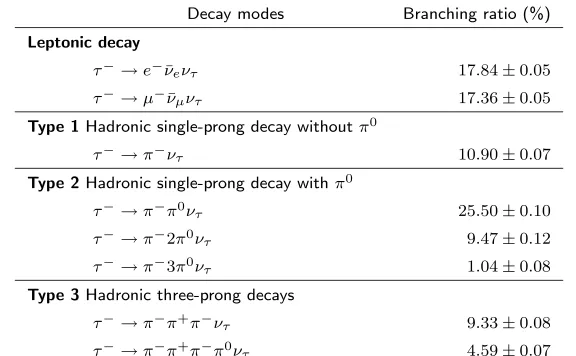
Table 2: Branching ratios (in unit of %) for dominant leptonic and hadronic decay modes of tau, sorted by expected tau type, as stated in Particle Data Book 2006 edition.

Decay modes Branching ratio (%)

Leptonic decay

τ− → _e−_ν¯_e_ν_τ 17_.84 ± 0_.05

τ− → _µ−_ν¯_µ_ν_τ 17_.36 ± 0_.05

Type 1 Hadronic single-prong decay without π0

τ− → _π−_ν_τ 10_.90 ± 0_.07

Type 2 Hadronic single-prong decay with π0

τ− → _π−_π0_ν_τ 25_.50 ± 0_.10

τ− → _π−2_π0_ν_τ 9_.47 ± 0_.12

τ− → _π−3_π0_ν_τ 1_.04 ± 0_.08

Type 3 Hadronic three-prong decays

τ− → _π−_π+_π−_ν_τ 9_.33 ± 0_.08

(23)

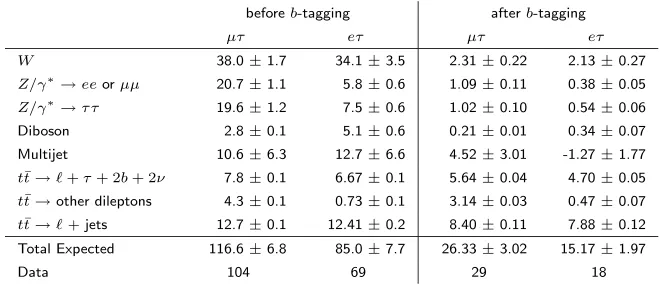
Table 3: Data and predicted numbers of events before and after b-tagging is applied. Standard model cross section and branching ratios are assumed for tt¯ production. Uncertainties are statistical only.

before b-tagging after b-tagging

µτ eτ µτ eτ

W 38.0 ± _1.7 _34.1 ± _3.5 _2.31 ± _0.22 _2.13 ± _0.27

Z/γ∗ _→ _ee _or _µµ _20.7 _± _1.1 _5.8 _± _0.6 _1.09 _± _0.11 _0.38 _± _0.05

Z/γ∗ _→ _{τ τ} _19.6 _± _1.2 _7.5 _± _0.6 _1.02 _± _0.10 _0.54 _± _0.06

Diboson 2.8 ± _0.1 _5.1 ± _0.6 _0.21 ± _0.01 _0.34 ± _0.07

Multijet 10.6 ± _6.3 _12.7 ± _6.6 _4.52 ± _3.01 _-1.27 ± _1.77

t¯t → _ℓ ₊ _τ _{+ 2}_b _{+ 2}_ν _7.8 ± _0.1 _6.67 ± _0.1 _5.64 ± _0.04 _4.70 ± _0.05

t¯t → _{other dileptons} _4.3 ± _0.1 _0.73 ± _0.1 _3.14 ± _0.03 _0.47 ± _0.07

t¯t → _ℓ _{+ jets} _12.7 ± _0.1 _12.41 ± _0.2 _8.40 ± _0.11 _7.88 ± _0.12

Total Expected 116.6 ± _6.8 _85.0 ± _7.7 _26.33 ± _3.02 _15.17 ± _1.97

(24)

Table 4: Systematics for the measurement of σ_t_t¯.

µτ eτ combined

∆σ ∆σ ∆σ

Jet energy calibration +0.30 −₀_.₅₀ _+0.33 −₀_.₃₆ _+0.43 −₀_.₃₅

PV identification +0.36 −₀_.₃₄ _+0.23 −₀_.₃₇ _+0.38 −₀_.₂₁

Muon identification +0.21 −₀_.₂₀ _– _+0.12 −₀_.₁₂

Electron identification – +0.59 −₀_.₅₃ _+0.25 −₀_.₂₄

Tau identification +0.16 −₀_.₁₅ _+0.15 −₀_.₁₅ _+0.16 −₀_.₁₆

Trigger +0.00 −₀_.₀₀ _+0.12 −₀_.₀₇ _+0.14 −₀_.₁₃

Fakes +0.45 −₀_.₄₂ _+0.59 −₀_.₅₃ _+0.50 −₀_.₄₉

b-tagging +0.31 −₀_.₃₄ _+0.44 −₀_.₄₁ _+0.45 −₀_.₃₇

MC normalization +0.18 −₀_.₁₈ _+0.15 −₀_.₁₅ _+0.13 −₀_.₁₃

Background/MC statistics +1.46 −₁_.₄₆ _+1.19 −₁_.₁₉ _+1.00 −₀_.₉₁

Other +0.08 −₀_.₀₈ _+0.09 −₀_.₁₀ _+0.19 −₀_.₁₈

Subtotal +1.76 −₁_.₆₇ _+1.64 −₁_.₅₉ _+1.40 −₁_.₂₄

Luminosity ±₀_.₄₉ ±₀_.₅₂ ±₀_.₅₁

(25)

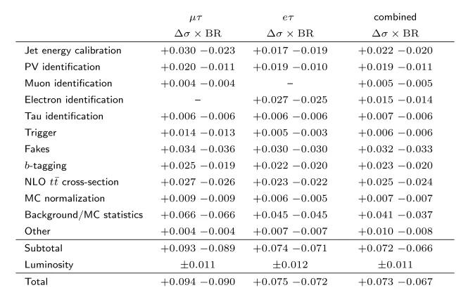
Table 5: Systematics for the measurement of σ_t_t¯× BR.

µτ eτ combined

∆σ × _BR _∆_σ × _BR _∆_σ × _BR

Jet energy calibration +0.030 −₀_.₀₂₃ ₊₀_.₀₁₇ −₀_.₀₁₉ ₊₀_.₀₂₂ −₀_.₀₂₀

PV identification +0.020 −₀_.₀₁₁ ₊₀_.₀₁₉ −₀_.₀₁₀ ₊₀_.₀₁₉ −₀_.₀₁₁

Muon identification +0.004 −₀_.₀₀₄ _– ₊₀_.₀₀₅ −₀_.₀₀₅

Electron identification – +0.027 −₀_.₀₂₅ ₊₀_.₀₁₅ −₀_.₀₁₄

Tau identification +0.006 −₀_.₀₀₆ ₊₀_.₀₀₆ −₀_.₀₀₆ ₊₀_.₀₀₇ −₀_.₀₀₆

Trigger +0.014 −₀_.₀₁₃ ₊₀_.₀₀₅ −₀_.₀₀₃ ₊₀_.₀₀₆ −₀_.₀₀₆

Fakes +0.034 −₀_.₀₃₆ ₊₀_.₀₃₀ −₀_.₀₃₀ ₊₀_.₀₃₂ −₀_.₀₃₃

b-tagging +0.025 −₀_.₀₁₉ ₊₀_.₀₂₂ −₀_.₀₂₀ ₊₀_.₀₂₃ −₀_.₀₂₀

NLO t¯t cross-section +0.027 −₀_.₀₂₆ ₊₀_.₀₂₃ −₀_.₀₂₂ ₊₀_.₀₂₅ −₀_.₀₂₄

MC normalization +0.009 −₀_.₀₀₉ ₊₀_.₀₀₆ −₀_.₀₀₅ ₊₀_.₀₀₇ −₀_.₀₀₇

Background/MC statistics +0.066 −₀_.₀₆₆ ₊₀_.₀₄₅ −₀_.₀₄₅ ₊₀_.₀₄₁ −₀_.₀₃₇

Other +0.004 −₀_.₀₀₄ ₊₀_.₀₀₇ −₀_.₀₀₇ ₊₀_.₀₁₀ −₀_.₀₀₈

Subtotal +0.093 −₀_.₀₈₉ ₊₀_.₀₇₄ −₀_.₀₇₁ ₊₀_.₀₇₂ −₀_.₀₆₆

Luminosity ±₀_.₀₁₁ ±₀_.₀₁₂ ±₀_.₀₁₁