77
MODELLING THE NUMBER OF NEW PULMONARY
TUBERCULOSIS CASES WITH GEOGRAPHICALLY WEIGHTED
NEGATIVE BINOMIAL REGRESSION METHOD
*Tsuraya Mumtaz
1‡and Agung Priyo Utomo
21Majoring in Statistics, Sekolah Tinggi Ilmu Statistik, Indonesia, [email protected] 2Majoring in Statistics, Sekolah Tinggi Ilmu Statistik, Indonesia, [email protected]
‡corresponding author
Indonesian Journal of Statistics and Its Applications (eISSN:2599-0802) Vol 2 No 2 (2018), 77 - 92
Copyright © 2018 Tsuraya Mumtaz and Agung Priyo Utomo. This is an open-access article distributed under the Creative Commons Attribution License, which permits unrestricted use, distribution, and reproduction in any medium, provided the original work is properly cited.
Abstract
Tuberculosis (TB) is an infectious disease caused by Mycobacterium Tuberculosis. Untill now, TB is still one of the main problems in many countries, especially developing countries. Indonesia ranked second as the country with the highest TB cases in the world in 2015, where most cases were found in Java. This study was conducted to model the number of new pulmonary TB cases in Java by considering the spatial aspects using Geographically Weighted Negative Binomial Regression (GWNBR). GWNBR method was chosen because the data used in this study were overdispered. The result showed that the population density and percentage of healthy homes were not significantly influential in each region. While the number of community health center (Puskesmas) , the percentage of smokers, the percentage of households with good PHBS, the percentage of diabetes mellitus sufferer, and the percentage of people with less IMT were significant in some regions. In general, the GWNBR model was better for modelling the number of new pulmonary TB cases than negative binomial regression and GWPR.
Keywords: GWNBR, spatial, overdispersion, pulmonary tuberculosis.
1. Introduction
Tuberculosis is an infectious disease caused by Mycobacterium Tuberculosis. This bacteria is transmitted through the air (droplet nuclei) when a sputum from tuberculosis patient is inhaled by the others (Widoyono, 2008). Most of the tuberculosis bacteria attack the lung organ (90 percent), but can also attack other
organs (Suarni, 2009). This disease has been afflicted nearly by one-third of the
world’s population and stated as a Global Emergency by WHO. In 2015, 10.4 million
new pulmonary tuberculosis cases were found in the world and 10 percent among them have been died. Therefore, tuberculosis was considered as the second most deadly infectious disease in the world after HIV (World Health Organization, 2016).
In the same year, Indonesia rose to the second place as the country with the highest number of pulmonary tuberculosis cases in the world, reaching 10 percent of the total cases found. Pulmonary tuberculosis was even considered as a leading cause of the death for all age groups in Indonesia (Indonesian Health Research and Development Agency, 2014). The death victims caused by pulmonary tuberculosis is estimated at 61,000 people for each year (Ministry of Health, 2011). Pulmonary tuberculosis brought a lot of harm to the patient both on social and economic aspects. The pulmonary tuberculosis patients were estimated to lose about 3-4 months of their work time which resulting in 20-30 percent decline of household income in one year. In some cases, patients with pulmonary tuberculosis also experienced ostracism by the local community (Aditama, 2005). This indicates that pulmonary tuberculosis was one of the threats to the ideals of the nation, especially in achieving prosperity.
Pulmonary tuberculosis usually occurs in areas with large populations. In Indonesia, about 38 percent of pulmonary tuberculosis cases reported in 2015 occurred in densely populated provinces. The top three were West Java (59,446), East Java (49,824), and Central Java (39,593), where all of which located in Java Island. In addition to these three provinces, other provinces in Java such as Banten, DKI Jakarta, and Yogyakarta also had high rates of pulmonary tuberculosis (Ministry of Health, 2015).
The number of new pulmonary tuberculosis cases belongs to count data. Regression models that can be used to analyze the relationship between the predictor and the response variable in the form of count data are the negative Poisson and Binomial regression model. Poisson regression can be used only in the condition of equidispersion (variance of the response variable equal to its mean) (Cameron & Trivedi, 2013). However, this assumption is difficult to be fulfilled in reality. The variance of response variable is often greater than its mean (overdispersion). The alternative approach to overcome this overdispersion problem is by using the Binomial Negative Regression (McCullagh & Nelder, 1989).
Pulmonary tuberculosis-related studies were often associated with spatial aspects such as spatial dependencies and spatial heterogeneity. Spatial dependence can occur because pulmonary tuberculosis is a disease that can be transmitted easily and not limited to the administrative area. This is also in accordance with the law of geography by Tobler (Miller, 2004), which states that
Binomial Regression (GWNBR).
Based on the description above, this research was conducted to model the number of new pulmonary tuberculosis cases for each district / city in Java using GWNBR method. Indahwati and Salamah (2016) conducted a similar modeling in Surabaya using all sub-districts as their unit of analysis. However, the coverage of the area used was still too narrow and the characteristics of the observations were less diverse. Therefore, this research was conducted by using a wider coverage area that was districts/cities in Java Island. In addition, this study also presented a comparison between the GWNBR model and the model generated from other commonly used methods such as negative binomial regression and GWPR.
2. Methodology
2.1 Material and Data
This research used the secondary data consisting of one response variable and seven predictor variables, with the following details:
Table 1. Research Variables and The Data Source
No. Variable Source
1. The number of new pulmonary tuberculosis cases for each district/city in Java in 2013 (New cases: A case of pulmonary
tuberculosis that occurred during the last year before the enumeration) (Y)
Publication of Basic Health Research (Riskesdas) 2013 for every Province in Java
2. Population density of each district/city in Java in 2013 (X1)
Provincial Publication in Figures 2014 for each province in Java
3. The percentage of healthy houses for each district/city in Java in 2013 (X2)
Publication of Health Profile 2013 for each province in Java 4. The number of community health center
(Puskesmas) for each district/city in java in 2013 (X3)
Provincial Publication in Figures 2014 for each province in Java
5. The percentage of smokers for each district/city in Java in 2013 (X4)
Publication of Basic Health Research (Riskesdas) 2013 for every Province in Java
6. The percentage of households with clean and healthy behavior (PHBS) for each district/city in Java in 2013 (X6)
Publication of Health Profile 2013 for each province in Java
7. The percentage of people with diabetes mellitus for each district/city in Java in 2013 (X5)
Publication of Basic Health Research (Riskesdas) 2013 for every Province in Java
8. The percentage of people with less IMT value for each district/city in Java in 2013 (X7)
2.2 Analysis Method
Poisson Regression
Poisson regression is a nonlinear regression to model the relationship between response (count) and predictor variables with assumption that response variable (Y)
follows Poisson distribution with parameter μ and y = 0,1,2, ... .
The Poisson distribution has the same mean and variance, as follows:
E(Y) = Var(Y) =μ (1)
The link function for Poisson regression is: (McCullagh & Nelder, 1989)
𝜂𝑖 = log(𝜇𝑖) = 𝒙𝒊𝑇𝜷 = ∑𝑝𝑗=0𝑥𝑖𝑗𝛽𝑗 for i = 1,2,...,n and j = 0,1, 2,...,p (2)
So that Myers (1990) stated Poisson regression model as:
𝑦𝑖 = 𝜇𝑖 + ɛ𝑖 = 𝑒𝒙𝒊𝑇𝜷+ ɛ𝑖 = 𝑒∑𝑝𝑗=0𝑥𝑖𝑗𝛽𝑗+ ɛ𝑖 (3)
with ɛ𝑖 as an error parameter for the i-th observation and 𝜇𝑖 is the expectation value of 𝑦𝑖.
Overdispersion
Indications of overdispersion or underdispersion can be easily found by comparing the mean and variance of the response variables. Overdispersion occurs when the variance is greater than the average (Hilbe, 2011). Furthermore, in Hilbe (2011) also mentioned that overdispersion can be seen by dividing Pearson
Chi-square dispersion value or deviance by degrees of freedom. Let θ be the dispersion parameter of the divison result, then θ>1 means overdispersion, θ<1 means underdispersion, while θ=1 indicates the condition of equidispersion.
Negative Binomial Regression
According to HIlbe (2011), data with overdispersion can be overcome by involving a parameter derived from gamma distribution in the Poisson model mean. This process will produce a Poisson-Gamma distribution (mix) which similar to the Negative Binomial Distribution. The parameter values of the Poisson-Gamma
distribution are expressed in the form of μ = αβ and θ = 1 𝛼⁄ so the mean and variance can be stated as:
E[Y] = μ and V[Y] = μ+ θμ2 (4)
The Binomial Negative density function will be:
𝑓(𝑦; 𝜇, 𝜃) = Γ(𝑦+1)Γ(1 𝜃Γ(𝑦+1 𝜃⁄ )⁄ ) (1+𝜃𝜇1 )1𝜃 ( 𝜃𝜇
1+𝜃𝜇)𝑦
(5)
Where y = 0,1,2,... and θ ≥ 0
Negative Binomial Regression model belongs to the Generalized Linear Model (GLM) group, so that in the estimation of the model coefficient parameter, the predictor variable can be written trough a linear combination with the natural logarithm link function as follows: (Hilbe, 2011).
𝑔(𝜇𝑖) = ln( 𝜇𝑖) = 𝒙𝒊𝑇𝜷 = ∑ 𝑥𝑖𝑗𝛽 𝑗 𝑘
𝑗=1
(6)
In the form of regression it can be written as:
𝑦𝑖 = exp(𝒙𝒊𝑇𝜷) + 𝜀𝑖 = exp (∑ 𝑥𝑖𝑗𝛽𝑗 𝑘
𝑗=1 ) + 𝜀𝑖
(7)
With 𝒙𝒊 as a vector of predictor variable, 𝜷 as a vector of regression coefficient, and
𝜀𝑖 as an error parameter of the i-th observation.
Spatial Dependency
Spatial dependency testing is performed to see if the observations at one location affect the observations in other adjacent locations. In general, inter-regional linkages can be measured using Moran's Index statistics. According to Anselin (1995), statistical tests that can be used to determine the existence of spatial dependence is Moran's Index test with the following hypothesis:
𝐻0: 𝐼 = 0 (No spatial dependency) 𝐻1: 𝐼 ≠ 0
Test statistics:
Zhit =√Var(Î)Î-E(Î) (8)
With I, E(𝐼̂), and Var(𝐼̂) as the Moran’s index value, expected value, and
variance. I can be written as the following:
𝐼̂ = 𝑛 ∑𝑛𝑖=1∑𝑛𝑗=1𝑤𝑖𝑗(𝑦𝑖−𝑦̅)(𝑦𝑗−𝑦̅)
(∑𝑛𝑖=1∑𝑛𝑗=1𝑤𝑖𝑗) ∑𝑛 (𝑦𝑖−𝑦̅)2 𝑖=1
(9)
Where:
n : number of observations
𝑦̅ : mean value of 𝑦𝑖 from n locations
𝑦𝑖 : observations value at the i-th location 𝑦𝑗 : observations value at the j-th location
𝑤𝑖𝑗 : the element of spatial weighting matrix
Decline 𝐻0 if |𝑍ℎ𝑖𝑡| > 𝑍𝛼 2⁄ , which means that there are spatial dependencies between response variables for each observation.
Spatial Heterogeneity
Characteristic differences between one observation point and other observation point lead to the spatial heterogeneity, so that the resulting regression parameters may vary. According to Anselin (1998), testing of spatial heterogeneity can be done using Breusch-Pagan with the following hypothesis:
𝐻0: 𝜎12 = 𝜎22 = ⋯ = 𝜎𝑛2 = 𝜎2 (Spatial homogeneity) 𝐻1: At least one 𝜎𝑖2 ≠ 𝜎2
Breusch-Pagan (BP) test statistics:
BP = (1 2⁄ ) 𝒇𝑻𝒁(𝒁𝑻𝒁)−1𝒁𝑻𝒇 (10)
where:
f = (𝑓1, 𝑓2, … , 𝑓𝑛)𝑇 𝑑𝑒𝑛𝑔𝑎𝑛 𝑓𝑖 = (𝑒𝑖2
𝜎2 − 1)
𝑒𝑖 = 𝑦𝑖 − 𝑦̂𝑙
𝑒𝑖2 : error square of the i-th observation
𝒁 : an n(k+1) matrix containing a normally-standardized vector (z) for each
According to Fotheringham, et al (2002), the formation of a spatial weights matrix can be performed using two kernel functions based on its bandwidth, that are the fixed and adaptive kernel function.
1. Fixed Kernel Function
This approach is suitable to be applied to the area with adjacent locations and less suitable to be applied to areas with remote locations. In this function, one optimum bandwidth value is applied to the whole area of observation.
- Fixed Gaussian Kernel Function
𝑤𝑖𝑗 = 𝑒𝑥𝑝 [−12 (𝑑𝑏 )𝑖𝑗 2
] (11)
- Fixed Bi-square Kernel Function
𝑤𝑖𝑗 = {[1 − (𝑑𝑏𝑖𝑗) nearest neighbors. This functionality applies relatively small bandwidth to adjacent areas and relatively large bandwidth in remote areas.
The adaptive kernel function can be divided into two following functions:
- Adaptive Gaussian Kernel Function
wij = exp [-12(bdi(q)ij ) 2
] (13)
- Adaptive Bi-square Kernel Function
𝑤𝑖𝑗 = {[1 − ( (𝑢𝑗, 𝑣𝑗) which are calculated by the following equation:
𝑑𝑖𝑗 = √(𝑢𝑖 − 𝑢𝑗)2+ (𝑣𝑖 − 𝑣𝑗)2 (15)
Where l(𝜃 ̂ |𝑦) is the maximum value from log-likelihood model and p is the number of parameters in the model including the constant.
Geographically Weighted Poisson Regression (GWPR)
GWPR is a development model of Poisson regression with local parameter estimator and the assumption of Poisson-distributed data. In this model the regression coefficients are influenced by the geographic location symbolized as
(𝑢𝑖, 𝑣𝑖) being the location where the data is observed. The GWPR model can be
described as follows:
𝑦𝑖~Poisson (𝑢𝑖) , where 𝐸[𝑦𝑖 ] = 𝜇𝑖̃ = exp(∑𝑝𝑗=0𝛽𝑗(𝑢𝑖, 𝑣𝑖)𝑥𝑖𝑗), for i=1,2,...,n and j=1,2,...,p
with:
k : number of predictor variables
𝑦𝑖 : the response value of the i-th observation
𝑥𝑖𝑗 : the observation value of the k-th predictor variable at the observation coordinate (𝑢𝑖, 𝑣𝑖)
𝛽𝑗(𝑢𝑖, 𝑣𝑖) : regression coefficient of the j-th predictor variable at the observation
coordinate (𝑢𝑖, 𝑣𝑖)
(𝑢𝑖, 𝑣𝑖) : the latitude and longitude coordinates of the i-th point at a geographic
location
Geographically Weighted Negative Binomial Regression (GWNBR)
The GWNBR model is a method used to model data counts that have spatial dependency and heterogeneity when overdispersion occurs in the data. This model will provide different local parameter estimates for each location. GWNBR is an extension of a global model that allows spatial variation of parameters 𝛽𝑘 and 𝜃. The local model of GWNBR can be written as follows (Da Silva, 2013):
𝑦𝑖 ~𝑁𝐵[ exp (∑ 𝛽𝑗 𝑗(𝑢𝑖, 𝑣𝑖)𝑥𝑖𝑗) , 𝜃(𝑢𝑖, 𝑣𝑖)] with i = 1,2,..., n (17)
Where (𝑢𝑖, 𝑣𝑖) is the coordinate of i-th observation. In regression form can be written as follows:
𝐸[𝑦𝑖 ] = 𝜇𝑖̂ = exp{(𝛽0𝑢𝑖, 𝑣𝑖) + ∑ 𝛽𝑗(𝑢𝑖, 𝑣𝑖)𝑥𝑖𝑗 𝑗
+ 𝜃(𝑢𝑖, 𝑣𝑖)} (18)
Where :
𝑦𝑖 : the value of the i-th observation
𝑥𝑖𝑗 : the observation value of the k-th predictor variable at the observation
coordinate (𝑢𝑖, 𝑣𝑖)
𝛽𝑗(𝑢𝑖, 𝑣𝑖) : regression coefficient of the j-th predictor variable at the observation
coordinate (𝑢𝑖, 𝑣𝑖)
𝜃(𝑢𝑖, 𝑣𝑖) : dispersion parameter of location (𝑢𝑖, 𝑣𝑖)
ln 𝐿(. ) = ∑𝑛𝑖=1𝑤𝑖𝑗(𝑢𝑖, 𝑣𝑖) [lnΓ(1 𝜃Γ(𝑦⁄ 𝑖𝑖+1 𝜃) Γ(𝑦⁄ 𝑖𝑖+1)) + 𝑦𝑖ln(𝜃𝑖𝜇𝑖) − (1 𝜃⁄ +𝑖
𝑦𝑖) ln (1 + 𝜃𝑖𝜇𝑖)] (19)
With 𝐿(. ) = 𝐿(𝜷(𝑢𝑖, 𝑣𝑖), 𝜃𝑖|𝑥𝑖𝑗, 𝑦𝑖) and 𝜇𝑖 = exp(𝒙′𝑖𝜷(𝒖𝒊, 𝒗𝒊))
Parameter estimation process is done by using the MLE method with Newton-Raphson numeric iteration. This method will use the information from Hessian matrix until the results are convergent.
GWNBR Model Parameter Test
Parameter testing can be done either simultaneously or partially. Simultaneous test aims to see whether or not all predictor variables influence the response variable together. The test hypothesis used is:
𝐻0 : 𝛽1(𝑢𝑖, 𝑣𝑖) = 𝛽2(𝑢𝑖, 𝑣𝑖) = 𝛽3(𝑢𝑖, 𝑣𝑖) = ... = 𝛽𝑘(𝑢𝑖, 𝑣𝑖) = 0
𝐻1 : at least one 𝛽𝑗(𝑢𝑖, 𝑣𝑖)≠ 0 , for j= 1,2,...,k
Test Statistic:
𝐺 = −2ln [𝐿(𝜔𝐿(Ω̂̂] ~ 𝜒(𝑘)2 (20)
𝐿(𝜔̂) is a likelihood value for a set of parameter under 𝐻0(intercept only), while
𝐿(Ω̂) is a likelihood value for the model with all predictor variables in. The decision will be taken is reject 𝐻0 if G>𝜒(𝛼,𝑘)2 , which indicates that there is at least one of GWNBR parameter that has a significant effect on the response variable.
Partial test is done to know which parameter have a significant effect to the response variable in each location. Testing parameters GWNBR model partially using the z-score test with the following hypothesis:
𝐻0 : 𝛽𝑗(𝑢𝑖, 𝑣𝑖) = 0 , for j= 1,2,...,k
𝐻1 : 𝛽𝑗(𝑢𝑖, 𝑣𝑖)≠ 0
Test statistics:
𝑍 = 𝛽̂𝑗(𝑢𝑖,𝑣𝑖)
𝑠𝑒(𝛽̂𝑗(𝑢𝑖,𝑣𝑖)) ~ N(0,1) (21)
With 𝛽̂𝑗(𝑢𝑖, 𝑣𝑖) is the estimated parameter 𝛽𝑗(𝑢𝑖, 𝑣𝑖) and 𝑠𝑒(𝛽̂𝑗(𝑢𝑖, 𝑣𝑖)) is the estimated standard error from diagonal element of covariance (𝛽̂𝑗(𝑢𝑖, 𝑣𝑖)) matrix. Reject 𝐻0 if |𝑍ℎ𝑖𝑡𝑢𝑛𝑔| > 𝑍𝛼 2⁄ which indicates that parameter 𝛽𝑗(𝑢𝑖, 𝑣𝑖) has significant effect on the response variable.
GWNBR Model Evaluation
Model evaluation is conducted to find out which model is more effective to model the response variable. Evaluation is done by comparing the model based on deviance value and AIC. According to Gill (2001) model evaluation based on deviance can use the following equation:
𝐷 = −2 𝑙𝑛 [𝐿(𝑦|𝛽̂𝐿(𝑦|𝜇̂)∗(𝑢𝑖, 𝑣𝑖)]
= 2 ∑𝑛𝑖=1[𝑦𝑖ln (𝜇̂𝑖(𝑢𝑦𝑖𝑖,𝑣𝑖)) + (1 + 𝑦𝑖)𝑙𝑛 (1+𝜇̂1+𝑦𝑖(𝑢𝑖𝑖,𝑣𝑖))]
With ln 𝐿(𝑦|𝛽̂∗(𝑢𝑖, 𝑣𝑖) as a natural logarithm of the model estimation without involving the predictor variable at location i and ln 𝐿(𝑦|𝜇̂) as a natural logarithm of the model estimation by involving all the predictor variables at location i. The smaller the deviance value the less error generated by the model (McCullagh & Nelder, 1989).
In addition to deviance, Akaike Information Criterion (AIC) is often used as a criterion in determining the best model. Basically the best model is a model that minimizes the sum of the negative likelihood values and the number of parameters used (AIC).
3. Results and Discussion
3.1 Characteristics and Distribution Pattern of The Number of New Pulmonary Tuberculosis Cases in Java in 2013
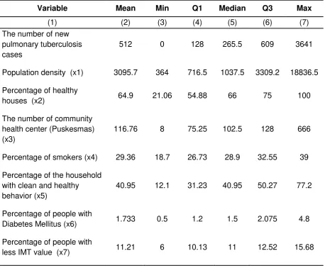
Transmission of pulmonary tuberculosis that could occur easily caused the disease was often associated with other factors, whether environmental factors, behavior, and individual immunity itself. Table 1 presented the descriptive statistics of the number of new pulmonary tuberculosis cases and the variables suspected to be influential.
Table 2. Descriptive Statistics of The Number of New Pulmonary Tuberculosis Cases in Java in 2013 and Related Variables
Variable Mean Min Q1 Median Q3 Max
(1) (2) (3) (4) (5) (6) (7)
The number of new pulmonary tuberculosis cases
512 0 128 265.5 609 3641
Population density (x1) 3095.7 364 716.5 1037.5 3309.2 18836.5
Percentage of healthy
houses (x2) 64.9 21.06 54.88 66 75 100
The number of community health center (Puskesmas) (x3)
116.76 8 75.25 102.5 128 666
Percentage of smokers (x4) 29.36 18.7 26.73 28.9 32.55 39
Percentage of the household with clean and healthy behavior (x5)
40.95 12.1 31.23 40.95 50.27 77.2
Percentage of people with
Diabetes Mellitus (x6) 1.733 0.5 1.2 1.5 2.075 4.8
Percentage of people with
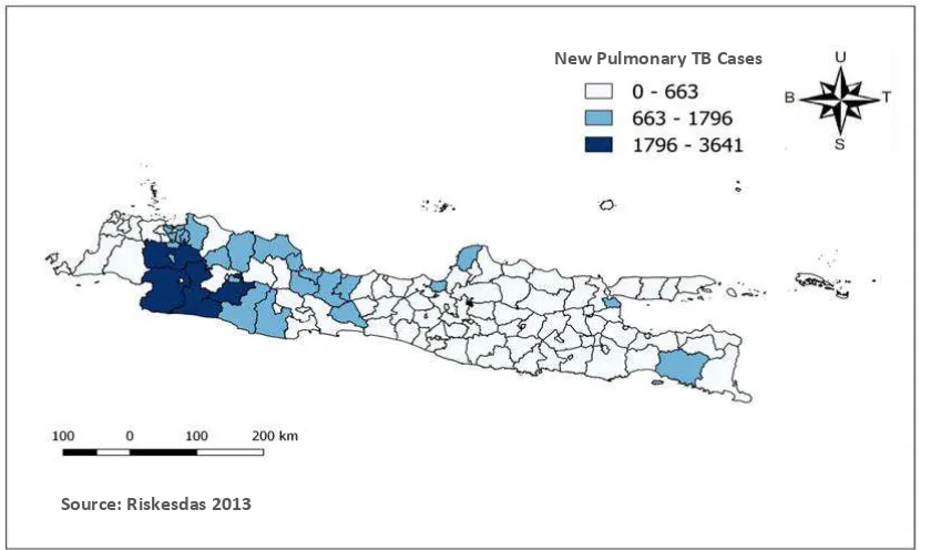
Figure 1. Distribution Map of The Number of New Pulmonary Tuberculosis Cases in Java in 2013.
The diversity of regional characteristics owned by each district/city causes the number of new pulmonary tuberculosis cases found to be various as well. In Figure 1 above, a map of the new pulmonary tuberculosis cases distribution for each district/city in Java was presented.
In 2013, there were found about 60,411 new pulmonary tuberculosis cases in Java with the most cases occurred in Bogor regency which reached 3,641 cases. Meanwhile, there were four regencies / cities with zero new cases such as Pamekasan Regency, Bondowoso Regency, Surakarta City, and Blitar City. This might happen because the data collection was done by survey so that new pulmonary tuberculosis cases could not be collected as a whole.
3.2 Overdispersion
Before conducting dispersion testing, multicollinearity assumption checks were necessary to select the variables to be used. Violations on this assumption of multicollinearity would cause standard deviation of the regression coefficients to be insignificant, making it difficult to separate the influence of each independent variable. Multicollinearity checks were performed using the Variance Inflation Factor (VIF) value. The result of the examination showed that there was no predictor variable that had VIF value more than 5. It meant there was no significant linear relationship between the predictor variable so that this assumption was fulfilled and the seven predictor variables could be used in the analysis.
Then, dispersion testing was done by using Rstudio 3.3.2 program. The result showed that with 𝑍0.05 = 5.7469 and p-value of 4.545e-09, the null hypothesis would be rejected. The conclusion was there was overdispersion in the data with dispersion
New Pulmonary TB Cases
parameter of 382.0079. Those situation caused the Poisson regression to be no longer suitable for modeling the data because the estimated parameters generated would be biased.
3.3 Modeling The Number of New Pulmonary Tuberculosis Cases with Negative Binomial Regression
The regression model that could be used to model the overdispersed data count was the Binomial Negative regression. Here were the results of modeling the number of new pulmonary tuberculosis cases with negative binomial regression.
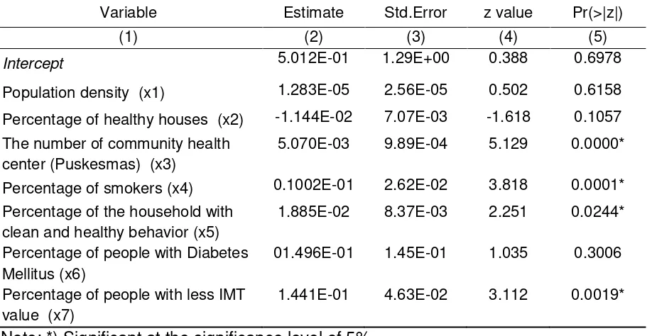
Table 3. Negative Binomial Regression Model of The Number of New Pulmonary Tuberculosis Cases
Variable Estimate Std.Error z value Pr(>|z|)
(1) (2) (3) (4) (5)
Intercept 5.012E-01 1.29E+00 0.388 0.6978
Population density (x1) 1.283E-05 2.56E-05 0.502 0.6158
Percentage of healthy houses (x2) -1.144E-02 7.07E-03 -1.618 0.1057 The number of community health
center (Puskesmas) (x3)
5.070E-03 9.89E-04 5.129 0.0000*
Percentage of smokers (x4) 0.1002E-01 2.62E-02 3.818 0.0001* Percentage of the household with
clean and healthy behavior (x5)
1.885E-02 8.37E-03 2.251 0.0244*
Percentage of people with Diabetes Mellitus (x6)
01.496E-01 1.45E-01 1.035 0.3006
Percentage of people with less IMT value (x7)
1.441E-01 4.63E-02 3.112 0.0019*
Note: *) Significant at the significance level of 5%
The table above showed that at the 0.05 significance level, the number of community health centers, the percentage of smokers, the percentage of households with clean and healthy behavior, and the percentage of people with less IMT value were not significantly affecting the number of new pulmonary tuberculosis cases.
3.4 Spatial Aspects Test
Next was the heterogeneity test performed by Breusch Pagan test. By using the Rstudio 3.3.2, statistical value of Breusch Pagan test resulted was 34.758 with p-value = 4.802e-06. Thus, at the level of significance of 0.05 it could be concluded that there is spatial heterogeneity between observation areas.
3.5 Modeling The Number of New Pulmonary Tuberculosis Cases with GWNBR
Modeling with Geographically Weighted Negative Binomial Regression began by calculating the spatial weights matrix. To obtain a spatial weights matrix, the bandwidth must first be determined. Determination of bandwidth was done by Golden Section Search technique. Bandwidth calculations required a matrix of distance between districts/cities. The distance used in this study was Euclidean distance with the selected bandwidth value was 101.82. The euclidean distance and bandwidth generated were then used to calculate the spatial weights matrix. Spatial weights matrix calculation was performed by using the Fixed Gaussian kernel function because it produced the smallest AIC value.
After the spatial weights matrix was obtained, the next step was modeling using GWNBR. To obtain a convergent parameter, iteration was done 20 times for each region. The GWNBR model generated 944 coefficients estimates (𝛽̂ (𝑢𝑗 𝑖, 𝑣𝑖)) for 118 districts/cities in Java. The coefficient determined the magnitude of the changes in the response variables for each change of the predictor variables.
Furthermore, simultaneous testing was done by comparing the deviance model of GWNBR with 𝜒2(7,0.05) = 14.067. The deviance value of GWNBR model was 59.002. Because the deviance value was greater, then with a significance level of 0.05 it could be concluded that at least one of GWNBR parameter was significant in the model. After simultaneous testing was done, it was necessary to test partially to know which parameters were significant in the model. The partial test result showed that with significance level of 0.05 it could be concluded that not all local parameter coefficients were significant in the model. For example, the following model would be shown for Indramayu Regency (Regency/City Code: 3212):
𝜇̂3212 = exp(0.2808∗− 0.0000177𝑥1− 0.00619𝑥2+ 0.004521𝑥3+ 0.113298𝑥4∗ − 0.01552𝑥5 + 0.140496𝑥6∗ + 0.141361𝑥7∗+ 1.142317∗)
Note: *) significant at the significance level of 5%
Based on the model above it was known that the intercept coefficient and dispersion parameters (theta) were significant in the model. Intercept value of 0.2808 showed that when other variables were zero then the number of new pulmonary tuberculosis cases in Indramayu district was e0.2808~ 1 case. While the theta value of 1.142317 indicated an overdispersion in the data.
In addition, it also could be seen from the model that there were three significant predictor variables at the 0.05 significance level. For the percentage of smokers variable, it could be interpreted that every one percent increase of smokers, the number of new pulmonary tuberculosis cases would increase as much as 𝑒0.113298 =
cases would increase as much as 𝑒0.140496= 1.15084 times assuming that other variables were constant. The last for the percentage of people with less IMT value. it could be interpreted that every one percent increase of people with less IMT value. the number of new pulmonary tuberculosis cases would increase as much as
𝑒0.141361= 1.1518 times assuming that other variables were constant.
3.6 Grouping Areas
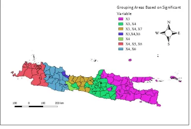
Modeling using GWNBR resulted the different parameter coefficients and 𝑍ℎ𝑖𝑡𝑢𝑛𝑔 for each region. This allowed a variable to has a significant effect in a particular area but was not significant in other regions. Therefore, grouping of regions based on significant variables needed to be done to identify areas with similar characteristics. Here were the grouping of regions based on significant variables.
Figure 2. Grouping Areas Based on Significant Variable
From the picture above could be seen that there were seven groups of districts/cities that were formed. The districts/cities in Banten, DKI Jakarta, and some of West Java entered in group 6 with three significant variables: percentage of smokers, percentage of households with clean and healthy behavior, and percentage of people with diabetes mellitus. While the district /cities in East Java and some districts/cities in Central Java entered in group 1 with only one significant variable that is the number of community health center. It also could be seen that only Cilacap regency that entered in group 5 with only one significant variable that is the percentage of smokers. Not only group 5, group 4 also only consisted of two areas, namely Cirebon regency and Banjar city.
3.8 Fitting the GWPR Model
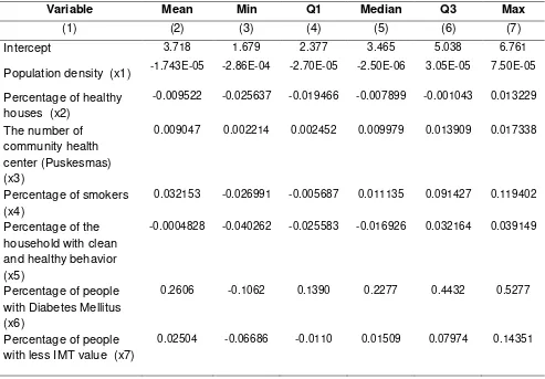
Data count modeling by considering spatial aspects could also be done using GWPR method with the assumption that there was no overdispersion in the data. The result of modeling using GWR4 showed that the parameter coefficient of GWPR model had negative to positive value ranges for six variables. That meant there were some areas with the parameter coefficients that were contrary to the theories already proposed. Table 4 showed a summary of the results.
Table 4. Summary of Modeling Results of New Pulmonary Tuberculosis Cases by GWPR
Variable Mean Min Q1 Median Q3 Max
(1) (2) (3) (4) (5) (6) (7)
Intercept 3.718 1.679 2.377 3.465 5.038 6.761
Population density (x1) -1.743E-05 -2.86E-04 -2.70E-05 -2.50E-06 3.05E-05 7.50E-05 Percentage of healthy
houses (x2)
-0.009522 -0.025637 -0.019466 -0.007899 -0.001043 0.013229
The number of community health center (Puskesmas) (x3)
0.009047 0.002214 0.002452 0.009979 0.013909 0.017338
Percentage of smokers (x4)
0.032153 -0.026991 -0.005687 0.011135 0.091427 0.119402
Percentage of the household with clean and healthy behavior (x5)
-0.0004828 -0.040262 -0.025583 -0.016926 0.032164 0.039149
Percentage of people with Diabetes Mellitus (x6)
0.2606 -0.1062 0.1390 0.2277 0.4432 0.5277
Percentage of people with less IMT value (x7)
0.02504 -0.06686 -0.0110 0.01509 0.07974 0.14351
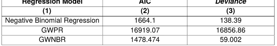
3.9 Evaluation of GWNBR Model
Table 5. AIC and Deviance Value of Negative Binomial Regression, GWPR, and GWNBR Model
It could be seen in Table 5 that the GWNBR model had smaller AIC and deviance values than other models. Therefore, it could be said that GWNBR method was better for modeling the number of new pulmonary tuberculosis cases in Java.
4. Conclusion and Suggestion
In 2013 there were found about 60,411 new cases of pulmonary tuberculosis in Java, with most cases found in Bogor district. In general, the distribution of those cases was not varied but forming certain groupings.
Modeling using GWNBR showed that with the significance level of 0.05 it could be concluded that the number of community health center and the percentage of smokers had a positive and significant influence in most districts. The percentage of households with clean and healthy behavior had a negative and significant influence in a small number of districts/cities (34.47%). While the percentage of people with diabetes mellitus and percentage of people with less IMT value had a positive and significant influence in a small number of districts/cities. Meanwhile, population density and percentage of healthy houses were not significant in the model for each district /city.
Over all, GWNBR method was better to model the overdispersed count data that had the spatial dependency and heterogeneity (in this case is the number of new pulmonary tuberculosis cases) than negative binomial regression and GWPR method. The further research can use other independence variables which has not been used in this research. Also, it is necessary to examine whether there are any specific spatial effect measurements for the count data.
References
Aditama, Y. (2005). Tuberkulosis dan Kemiskinan. Majalah Kesehatan Indonesia, 55(2) , 49-51.
Anselin, L. (1995). Local Indicators of Spatial Association-LISA. Geographical Analysis, 27 (2), 93-115.
Anselin, L. (1988). Spatial Econometric Methods and Model. Dordrecht: Kluwer Academic Publishers.
Cameron, A., & Trivedi, P. (2013). Regression Analysis of Count Data (Second ed).
Cambridge: Cambridge University Press.
Da Silva, A. & Rodrigues, T. (2013). Geographically Weighted Negative Binomial Regression: Incorporating Overdispersion. New York: Springer.
Fotheringham, A. S., Brunsdon, C., & Charlton, M. (2002). Geographically Weighted Regression. Inggris: University of Newcastle.
Gill, P. J. (2001). Generalized Linear Models: A Unified Approach. California: Sage Publication, Inc.
Hilbe, J. (2011). Negative Binomial Regression (2nd ed). New York: Cambridge University Press.
Indahwati, S. D. (2016). Analisis Faktor-Faktor yang Memengaruhi Jumlah Kasus Tuberkulosis di Surabaya Tahun 2014 Menggunakan Geographically Weighted Negative Binomial Regression. Jurnal Sains dan Seni ITS, 5(2), 193-197.
Kementerian Kesehatan RI. (2011). Strategi Nasional Pengendalian Tb di Indonesia Tahun 2010-2014. Jakarta: Kementerian Kesehatan RI.
McCullagh, P., & Nelder, J. (1989). Generalized Linear Models (Second ed). London: Chapman and Hall.
Miller, H. (2004). Tobler's First Law and Spatial Analysis. Annalys of the Association of American Geographers, 94(2), 284-289.
Myers, R. (1990). Classical and Modern Regression with Application Second Edition. New York: PWS-KENT.
Ramadhan, R. F. (2016). Pemodelan Data Kematian Bayi dengan Geographically Weighted Negative Binomial Regression. Media Statistika, 9(2), 95-106.
Suarni, H. (2009). Faktor Risiko yang Berhubungan dengan Kejadian Penderita Penyakit TB Paru BTA Positif di Kecamatan Pancoran Mas Kota Depok Bulan Oktober Tahun 2008-April Tahun 2009 [Skripsi] . Depok: FKM UI.
Widarjono, A. (2007). Ekonometrika Teori dan Aplikasi untuk Ekonomi dan Bisnis.
Yogyakarta: Ekonosia FE UII.
Widoyono. (2008). Penyakit Tropis: Epidemiologi, Penularan, Pencegahan, dan Pemberantasannya. Jakarta: Erlangga.