A
Analytical Details
A.1 HouseholdsCost Minimization Households decide the composition of the consumption basket to minimize expenditures
min {Ck
it}i
1
0
PitCitkdi
s.t.
1
0
Citk−θCit−1
η−1 η
di
η η−1
≥Xkt
The demand for individual goods iis
Citk =
Pit
Pt
−η
Xtk+θCit−1,
where Pt is the overall price level, expressed as an aggregate of the good i prices, Pt =
1 0 P
1−η it di
1 1−η
.
Utility Maximization The solution to the utility maximization problem is ob-tained by solving the Lagrangian function,
L=E0 ∞
t=0
βt uXk t, Ntk
−λk
t
PtXtk+Ptϑt+Qt,t+1Dt+1k −WtNtk(1−τ)−Dkt −Φt−Tt
In the budget constraint, we have re-expressed the total spending on the consumption basket,01PitCitkdi, in terms of quantities that affect the household’s utility,
1
0
PitCitkdi=PtXtk+Ptϑt,
where under deep habits ϑt is given as ϑt ≡ θ
1 0
Pit Pt
Cit−1di, while under superficial
habits it takes the simpler form,ϑt≡θCt−1. Households take ϑt as given when
maximiz-ing utility.
The first order conditions are then,
Xk t
: uX(t) =λktPt
Nk t
: −uN(t) =uX(t)WPtt(1−τ)
Dk t
: 1 =βEt uXu(t+1) X(t)
Pt Pt+1
Rt
where Rt= Et[Q1
t,t+1] is the one-period gross return on nominal riskless bonds.
With utility given by u(X, N) = X1−σ 1−σ −N
1+υ
1+υ , the first derivatives are
A.2 Firms
The cost minimization involves the choice of labor input Nit subject to the available
production technology
min
Nit
WtNit
s.t. AtNit=Yit
The minimization problem implies a labor demand, Nit = YAitt, and a nominal marginal
cost which is the same across all brand producing firms, M Ct = (1−κ)Wt
where the last term represents the nominal costs of adjusting prices, as in Rotemberg (1982), andπ is the steady state inflation.
Each firm then chooses processes for Pit and Yit to maximize the present discounted
value of profits, under the restriction that all demand be satisfied at the chosen price (Cit=Yit):
The first order conditions are:
vit= (Pit−M Ct) +θEt[Qt,t+1vit+1]
where vit is the Lagrange multiplier on the dynamic demand constraint and represents
B
Equilibrium Conditions
B.1 Aggregation and SymmetryAggregate output: In this setup, all firms and all households are symmetric. This implies that aggregate output is given by
Yt=AtNt
Aggregate resource constraint: Aggregate profits are
Φt=PtYt−WtNt−
ϕ
2 πt
π −1
2
PtYt
and the household budget constraint becomes in equilibrium (note: PtXt+Ptϑt reduces
to PtCt)
PtCt=WtNt(1−τ) + Φt+Tt
Combine the household budget constraint with the government budget constraint (τ WtNt=Tt)
and the definition of profits to obtain the aggregate resource constraint
Ct+
ϕ
2 πt
π −1
2
Yt=Yt
B.2 System of Non-linear Equations
Xt=Ct−θCt−1 (32)
NtυXtσ =
Wt
Pt
≡wt(1−τ) (33)
Xt−σ =βEt
Xt+1−σ Rtπ−1t+1
(34)
Yt=ηωtXt+ϕ
πt
π −1
πt
πYt−ϕβEt
Xt+1
Xt
−σ
πt+1
π −1
π
t+1
π Yt+1
(35)
ωt=
1− 1
μt
+θβEt
Xt+1
Xt
−σ
ωt+1
(36)
Yt=AtNt (37)
Yt=Ct+
ϕ
2 πt
π −1
2
Yt (38)
B.3 The Deterministic Steady State
The non-stochastic long-run equilibrium is characterized by constant real variables and nominal variables growing at a constant rate. The equilibrium conditions (32) - (41) reduce to:
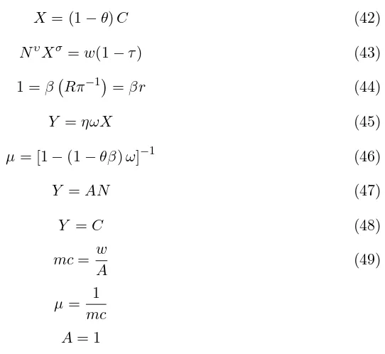
X = (1−θ)C (42)
NυXσ =w(1−τ) (43)
1 =βRπ−1=βr (44)
Y =ηωX (45)
μ= [1−(1−θβ)ω]−1 (46)
Y =AN (47)
Y =C (48)
mc= w
A (49)
μ= 1
mc A= 1
Table 1 contains the imposed calibration restrictions. We assume values for the real interest rate, the Frisch labor supply elasticity, steady state inflation, and the parameters
σ, η,ϕ, andθ. The discount factor β matches the assumed real rate of interest,β =r−1,
while the nominal interest rate isR=rπ. Given the specification of the utility function,
υ is the inverse of the Frisch labor supply elasticity, ǫN w = υ1.
With no price adjustment costs in the deterministic steady state,C =Y.Then, using equations (42) and (45), the steady state value of the shadow priceω is
ω = [η(1−θ)]−1,
while the markupμ is given by equation (46) and the marginal cost is its inverse,mc =
μ−1.
To determine the steady state value of labor, we substitute forXin terms ofY in (43) and then, using the aggregate production function, we obtain the following expression,
Nσ+υ[(1−θ)A]σ =w(1−τ), (50)
steady-state condition for marginal costs,mc=w/A= 1/μ
Nσ+υ[(1−θ)A]σ = A
μ(1−τ), (51)
In order for this condition to match the social planner’s allocation (65) it must be the case that τ = 1−μ(1−θβ). See Appendix E for the social planner’s problem. Finally, equations (47) and (42) can be solved for aggregate output Y (or consumption C) and habit-adjusted consumptionX.
B.4 System of Log-linear Equations
Log-linearizing the equilibrium conditions (32) - (41) around the efficient deterministic steady state gives the following set of equations:
Xt= (1−θ)−1
Ct−θCt−1
σXt+υNt=wt
Xt=EtXt+1−
1
σ
Rt−Etπt+1
Yt=ωt+Xt+ϕ(πt−βEtπt+1) (52)
ωt=
1
μωμt+θβEtωt+1+θβσ
Xt−EtXt+1
(53)
Yt=At+Nt
Yt=Ct
mct=wt−At
μt=−mct
At=ρAt−1+εt
The New Keynesian Phillips Curve is given by the pricing equation (52)
πt=βEtπt+1+ 1
ϕ
Yt−ωt−Xt
C
The Case of Superficial External Habits
C.1 HouseholdsHabits are “superficial” when they are formed at the level of the aggregate consumption good. Households derive utility from the habit-adjusted composite goodXtk,
Xtk=Ctk−θCt−1,
where household k’s consumption, Ck
t, is an aggregate of a continuum of final goods,
indexed byi∈[0,1],
Ctk= 1
0
Citk
η−1 η
di
η η−1
,
with η >1 the elasticity of substitution between them and Ct−1 ≡01Ct−1k dk the
cross-sectional average of consumption.
Cost Minimization Households decide the composition of the consumption basket to minimize expenditures
min {Ck
it}i
1
0
PitCitkdi
s.t.
1
0
Citk
η−1 η
di
η η−1
≥Ckt.
The demand for individual goods iis
Citk =
Pit
Pt
−η
Ctk,
wherePt≡
1 0 P
1−η it di
1 1−η
is the consumer price index. The overall demand for good i
is obtained by aggregating across all households
Cit=
1
0
Citkdk=
Pit
Pt
−η
Ct. (54)
Unlike in the case of deep habits, this demand is not dynamic.
C.2 Firms
price is set optimally to satisfy the following relationship:
1−η
1− 1
μt
Yt=ϕ
πt
π −1
πt
πYt−ϕβEt
Xt+1
Xt
−σπ t+1
π −1
πt+1
π Yt+1
.
(55)
C.3 Equilibrium
In this setup, we obtain the familiar looking New Keynesian Phillips Curve,
πt=βEtπt+1+
η−1
ϕ mct (56)
to which we add the IS curve,
Xt=EtXt+1−
1
σRt+
1
σEtπt+1, (57)
and two equations defining the habit-adjusted consumption and the real marginal cost,
Xt=
1 1−θ
Yt−θYt−1
(58)
D
The Case of Internal Habits
D.1 HouseholdsHabits are internal and superficial when they are formed at the level of the aggregate consumption bundle but households endogenize the effects of their current consumption choices on future utility. Each householdkderives utility from a habit-adjusted composite good Xk
t,
Xtk =Ctk−θCt−1k
whereCk
t is the time-t aggregate of a continuum of goods, indexed byi∈[0,1],
Ctk=
1
0
Citk
η−1 η
di
η η−1
with η >0 the elasticity of substitution between them, and Ck
t−1 is the previous period
consumption of household k. Since households are symmetric and, in this case, we also do not need to distinguish between individual and aggregate variables, in what follows we drop thek superscript.
Cost Minimization The households’ cost minimization problem yields a typical static demand for each goodi,
Cit=
Pit
Pt
−η
Ct
wherePt≡
1 0 P
1−η it di
1 1−η
.
Utility maximization The Lagrangian function is
L=E0 ∞
t=0
βt
(Ct−θCt−1)1−σ
1−σ −
Nt1+υ
1 +υ
−λt(PtCt+EtQt,t+1Dt+1−WtNt(1−τ)−Dt−Φt−Tt)
whereRt= Et[Q1t,t+1] is the one-period gross return on nominal riskless bonds.
Anticipat-ing that current consumption decisions affect the stock of habits enterAnticipat-ing into the future, the consumption Euler equation is given by,
Xt−σ−θβEtXt+1−σ =βEt
Xt+1−σ −θβEt+1Xt+2−σ Rt
πt+1
and the labor supply condition by,
(Nt)υ
Xt−σ−θβEtXt+1−σ
In log-linear form, the first order condition for labor and the Euler equation become
The firms’ behavior is unchanged, except that the stochastic discount factor in their profit maximization problem is given by,
Qt,t+s=βs
and the firms’ FOC for price is then
[1−η(1−mct)]Yt=ϕ
In a deterministic steady state, this relationship still reduces to 1 =η(1−mc),and the log-linearized equation, which is essentially the NKPC, is the same as under external superficial habits.
The marginal cost relationship is slightly modified due to the different marginal rate of substitution between consumption and labor:
Hence, the system of relevant equations includes the IS curve (61), the NKPC (56), the marginal cost relationship (62), and the usual definition of the habit-adjusted consumption (58).
In gap form
In the case of internal habits, it is easy to write these relationships in ‘gap’ form. Let
Ytg ≡Yt−Yt∗ andX g
t ≡Xt−Xt∗ denote the relevant ‘gap’ variables. Using the equations
as
and the NKPC is then,
The IS curve can also be written using gap variables and additional terms involving only the social planner’s allocation. From the social planner’s problem,X∗
t−θβEtXt+1∗ = 1−θβ
σ (1 +υ)At−υYt∗
, which then allows us to write the IS curve as (add and subtract the timet and (t+ 1) expressions from the LHS and RHS of the IS equation):
D.3 Optimal Policy: internal habits
In the case of internal (superficial) habits, we can show analytically that in response to technology shocks the Ramsey planner can set the nominal interest rate so as to match the social planner’s allocation, without creating inflation. Using the link between gap variables, Xtg = 1−θ1 Ytg−θYt−1g , we first express all relevant equations in terms of inflation and output gap. The welfare function Γ0 is
Γ0 =−
and the New Keynesian Phillips curve (63) is
With the IS curve not binding, the Lagrangian is
L=E0 ∞
t=0
βt
⎧ ⎪ ⎨ ⎪ ⎩
−12Ω
δYtg−θYt−1g 2+υYtg+ϕπ2t
−γt πt−βπt+1+η−1ϕ δ
θβEtYt+1g −ζYtg+θY g t−1
⎫ ⎪ ⎬ ⎪ ⎭
and the first order conditions for the output gap and inflation are:
Ytg : ζ
Ytg−η−1
ϕΩ γt
=θβEt
Yt+1g −η−1
ϕΩ γt+1
+θ
Yt−1g −η−1
ϕΩ γt−1
(πt) : πt=−
1
ϕΩ
γt−γt−1
with the additional restriction that, under full commitment, the central bank ignores past commitments in the first period and sets all pre-existing conditions to zero, Y−1g =
E
The Social Planner’s Problem
The subsidy level that ensures an efficient long-run equilibrium is obtained by comparing the steady state solution of the social planner’s problem with the steady state obtained in the decentralized equilibrium. The social planner ignores the nominal inertia and all other inefficiencies and chooses real allocations that maximize the representative consumer’s utility subject to the aggregate resource constraint, the aggregate production function, and the law of motion for habit-adjusted consumption:
max
{X∗ t,C∗t,Nt∗}
E0 ∞
t=0
βtu(Xt∗, Nt∗)
s.t. Yt∗ = Ct∗
Yt∗ = AtNt∗
Xt∗ = Ct∗−θCt−1∗
The optimal choice implies the following relationship between the marginal rate of sub-stitution between labor and habit-adjusted consumption and the intertemporal marginal rate of substitution in habit-adjusted consumption
χ(Nt∗)υ (X∗
t)−σ
=At
1−θβEt
X∗ t+1
X∗ t
−σ
.
The steady state equivalent of this expression can be written as,
χ(N∗)υ+σ[(1−θ)A]σ =A(1−θβ). (65)
The dynamics of this model are driven by technology shocks to the system of equilib-rium conditions composed of the Euler equation, the resource constraint, and the evolution of habit-adjusted consumption. In log-linear form, these are:
Xt∗ =θβEtXt+1∗ +
1−θβ σ
−υNt∗+At
Yt∗ =At+Nt∗
Xt∗ = 1 1−θ
Yt∗−θYt−1∗ ,
which combined yield the following dynamic equation
ζYt∗ =θβEtYt+1∗ +θYt−1∗ +
1 +υ
δ
At
where ζ ≡ 1 +θ2β+υ δ
and δ ≡ σ
(1−θβ)(1−θ). In the absence of deep habits,θ = 0, the
model reduces to the basic New Keynesian model where Y∗ t =
1+υ σ+υ
F
Derivation of Welfare
Individual utility in periodtis
Xt1−σ
1−σ − Nt1+υ
1 +υ
whereXt=Ct−θCt−1 is the habit-adjusted aggregate consumption. Before considering
the elements of the utility function, we need to note the following general result relating to second order approximations
Yt−Y
and O[2] represents terms that are of order higher than 2 in the bound on the amplitude of the relevant shocks. This will be used in various places in the derivation of welfare. Now consider the second order approximation to the first term,
Xt1−σ
where tip represents ‘terms independent of policy’. Using the results above this can be rewritten in terms of hatted variables
Xt1−σ
In pure consumption terms, the value ofXtcan be approximated to second order by:
To a first order,
Summing over the future,
∞
The term in labour supply can be written as
Now we need to relate the labor input to output which, in this case without price dispersion, is simply,
Nt=
Yt
At
and can be approximated to first order,
so we can then write
Nt1+υ
Welfare is then given by
Γ0 = X (1−θ)N1+υ. If we use the appropriate subsidy to render the steady-state efficient and also use the second order approximation to the national accounting identity,
we can eliminate the level terms and write the sum of discounted utilities as:
Γ0=−
welfare function as,
Summing across time periods, we have
E0
Then note that we can write
and, keeping only the terms relevant for policy, the welfare function becomes,
Γ0 =−1
Finally, we can show that
E0
which allows to write the welfare function in gap form as follows
Γ0 =−
F.1 Welfare Measure
We measure welfare as the unconditional expectation of lifetime utility, approximated as
withu the steady-state level of the momentary utility and the Λ coefficients defined as
The welfare terms associated with the Ramsey policy that are involved in computing the welfare costs of alternative policies, as in expression (28) in the text, are given by,
G
Optimal Policy: Commitment
Upon substitution of the habit-adjusted consumption term, the central bank’s objective function becomes
(1−θβ)(1−θ) and we re-write the constraints as,
respect to the nominal interest rate gives:
−σ−1E0βtχt= 0, ∀t≥0 (67)
which implies that the IS curve is not binding and it can therefore be excluded from the optimization problem. Once the optimal rules for the other variables have been obtained, we use the IS curve to determine the path of the nominal interest rate. So, the central bank now chooses "Yt,πt,ωt
#
The first order condition for the shadow value ωt gives the relationship between the two
Lagrange multipliers,
κ1ψt=−μω(ςt−θςt−1)
while for inflation we have the rather usual expression
The first order condition for output gives
−ΩδζYt+ΩδθYt−1+Ω (1 +υ)At−κ2ψt+γ2ςt−γ1ςt−1+βEt ΩδθYt+1+κ2ψt+1+γ3ςt+1
Under full commitment, the central bank ignores past commitments in the first period by setting all pre-existing conditions to zero, Y−1 = 0 and ψ−1 = ς−1 = 0. To find the
solution, solve the system of equations composed of the first order conditions, the three constraints, and the technology process.
G.1 Optimal Policy: Discretion
In order to solve the time-consistent policy problem we employ the iterative algorithm of Soderlind (1999), which follows Currie and Levine (1993) in solving the Bellman equation. The per-period objective function can be written in matrix form asZtQZt, whereZt+1 =
and the structural description of the economy is given by,
and
B0= 0 0 0 σ−1 0
.
−10 0 10
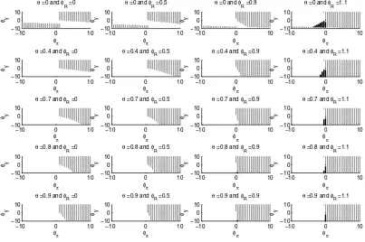
Figure 11: Determinacy properties of the model with internal habits, when monetary policy follows the rule Rt =φππt+φyYt+φRRt−1: determinacy (light grey dots),
inde-terminacy (blanks), and instability (dark grey stars).
0.1 0.2 0.3 0.4 0.5 0.6 0.7 0.8 0.9 5
10 15 20 25 30 35
θ
φ π
0.1 0.2 0.3 0.4 0.5 0.6 0.7 0.8 0.9−0.6
−0.4 −0.2 0 0.2 0.4 0.6 0.8 1 1.2
φ y
and
φ R
φπ
φ
y
φ
R
0.1 0.2 0.3 0.4 0.5 0.6 0.7 0.8 0.9 0
5 10 15 20 25 30 35 40 45 50
θ
φ π
0.1 0.2 0.3 0.4 0.5 0.6 0.7 0.8 0.9−0.5
0 0.5 1 1.5 2 2.5 3 3.5 4
φ y
and
φ R
φ
π
φ
y
φ
R
0 2 4 6 −0.05
0 0.05
Inflation
%
0 2 4 6
0 0.05 0.1
Output gap
0 2 4 6
−0.2 −0.1 0
Nominal interest rate
%
0 2 4 6
−0.2 −0.1 0
Real interest rate
0 2 4 6
0 0.2 0.4
Output
years
%
0 2 4 6
−0.5 0 0.5
Markup
years