VOL. 5, NO. 2, pp. 105-109, May, 2015
Numerical Study of Predator-Prey Model with Beddington-DeAngelis
Functional Response and Prey Harvesting
Fira Fitriah1
, Agus Suryanto1*
, Noor Hidayat2
1
Department of Mathematics, Faculty of Mathematics and Sciences, Universitas Brawijaya, 65145, Malang, Indonesia
ABSTRACT
A modified Leslie-Gower predator-prey model with Beddington-DeAngelis functional response and Michaelis-Menten type prey harvesting is studied. The equilibrium points of the system are investigated. To see the stability of each equilibrium point, we perform some numerical simulations. Our numerical simulations show that the extinction of prey or survival of both prey and predator are conditionally stable.
Keywords: harvesting, Leslie-Gower, Michaelis-Menten, numerical simulations, predator-prey model
Every species interact with other species in their habitat. Interactions between species lead to a rise or reduction population densities. Predation is one form of interaction between the two species (predator and prey). In the case of predation, a predator population density is increasing. In contrast, the density of the prey population is decreasing. Species compete, evolve, and spread for the aim of seeking the source of food to sustain their existence [1].
Environmental resources constrain the growth of each species. If the population density increases, the growth rate of population is reduced and stopped at a certain population density that is known as the carry-ing capacity. In other words, carrycarry-ing capacity is the maximum population density that can be supported by the environment [2].
In population dynamics, a functional response rep-resents the predation rate of prey by predators per capita. Holling [3] has introduced a functional re-sponse that depends only on the prey species, namely Holling type I, II, and III. Beddington [4] and DeAn-gelis [5] have modified the Holling functional re-sponse. Beddington and DeAngelis suggested that pre-dation rate is more realistic if it also depends on the predator species and environmental provides protection to the prey. Predator population densities are impor-tant to consider because the predators are competing
and sharing food.
Leslie [6] has introduced a predator-prey model with carrying capacity of the predator population is proportional to the number of prey population. The model is known as the Leslie-Gower predator-prey model. Aziz-Alaoui and Okiye [7] has modified the carrying capacity of the predator population in Leslie-Gower model. Aziz-Alaoui and Okiye involved the en-vironment protection. They used Holling-type II func-tional responses. The existence of the economic value of the prey population encourages modification by adding prey harvesting. Gupta and Chandra [8] has modified Aziz-Alaoui and Okiye model by incorporat-ing Michaelis-Menten type prey harvestincorporat-ing. Yu [9] has modified Aziz-Alaoui and Okiye model by the func-tional response into Beddington-DeAngelis-type.
In this article, we extend the predator-prey model proposed by Gupta and Chandra [8] and Yu [9] by in-corporating a Bedington-DeAngelis functional response and the Michaelis-Menten type prey harvesting. The focus of this study is to give an overview of population densities in the long term based on numerical simula-tions. Fourth order Runge-Kutta method is used to solve the predator-prey system.
Mathematical model
A mathematical model that represents the interac-tion between the prey species and the predator species will be constructed based on several assumptions. First, we assume that harvesting is performed only on prey species. Second, the coefficients of environmental pro-tection for the prey and predator population are
differ-MATERIALS AND METHODS INTRODUCTION
*Corresponding author: Agus Suryanto
Department of Mathematics, Faculty of Mathematics and Science, Universitas Brawijaya, 65145, Malang, Indonesia
ent.
Suppose x is the population density of prey and y is the population density of predator. It is assumed that prey grows with intrinsic growth rate r1 :
The existence of competition among prey species to survive in their habitat with competition rate p causing the prey population growth rate was reduced as follow
Based on Yu [9], the rate of predation is given in the form of the Beddington-DeAngelis functional response:
where α and ɑ are the maximum value of the per capita reduction rate of x due to y and the coefficient of environmental protection for the prey, respectively. b and c are suitable constants. Therefore, the prey population growth rate is reduced due to predation as follow
Harvesting prey by humans given in a nonlinear form, known as the Michaelis-Menten type as in Gupta and Chandra [8]. The prey population growth rate is re-duced due to harvesting as follow
where q is catchability coefficient, E is the effort
applied to harvest the prey species, and m1 and m2 are
suitable constants. m1E shows limited human effort to
harvest and m2x indicates the limited number of prey
that harvested. Based on the equation (1), (2), (3), and (4), the prey population growth rate is formulated as follow
with all parameters are positive constant.
It is assumed that predator grows with intrinsic
As Aziz-Alaoui and Okiye [7], the carrying capacity of the predator population is limited by prey population density and the extent to which the environmental pro-vides protection to predator (k). If β is the competition rate among predator species to survive in their habitat, the predator population growth rate is reduced as follow
Based on the equation (5) and (6), the predator popu-lation growth rate is formulated as follow
Thus, predator-prey models involving Beddington-DeAngelis functional response and Michaelis-Menten type prey harvesting is
Determination of the equilibrium point
The equilibrium point of the system (7) is the solu-tion of that system when both populasolu-tion growth rates are zero. Equilibrium point illustrates a constant solu-tion of the system.
Observing the stability of the equilibrium point Stability of the equilibrium point is observed by the Jacobian matrix of the system. The stability property shows whether the equilibrium point is stable or not. If the equilibrium point is stable, then any solution of the system with different initial values will be convergent to it, and vice versa.
Numerical experiments
in the long term. To determine the numerical solutions of the predator-prey model, we use the fourth order Runge-Kutta method.
Equilibrium Point
In order to find the equilibrium point of the system (7), let
where x and y have same meaning as x(t) and y(t), respectively. Obviously, system (7) has five equilibrium points, as follow.
i. The extinction of both prey and predator point E0 = (0,0)
ii. The predator extinction point E1 = (x*A, 0) and
E2 = (x*B, 0) where
iii. The prey extinction point E3 = (0, r2 k/ β)
iv. The positive equilibrium point E4 (x*, r2 (x* +
k)/β). x* is a positive real root of
where
In contrast to all of the equilibrium point, E4 (x*, r2
(x* + k)/β) shows that both the prey and the predator can survive in the long term.
Stability of Equilibrium Point
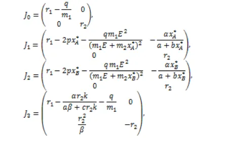
The Jacobian matrix of system (7) at equilibrium point (x,y) is
with
An equilibrium point (x,y) of system (7) is asymtotically stable if the real parts of all eigenvalues of J (x,y) are negative. The Jacobian matrices for E0, E1,
E2 and E3 are
respectively. r2 is a positive eigenvalue of J0, J1 and J2, so
E0, E1 and E2 are unstable equilibrium point. Therefore,
the extinction of both prey and predator or predator extinction does not occur in the long term. We next in-vestigate the stability of E3 and E4 by numerical
simula-tions.
Numerical Simulations
Let r1 = 0.3, a= 10, b = 1, c= 0.5, q= 0.3, E= 10, p=
0.05, m1= 0.1, α= 0.02, m2 = 0.6, r2= 0.2, β= 0.5 and RESULTS AND DISCUSSION
Figure 1. Numerical solution of system (7) with an asymptotically
k= 3. Based on those parameter values, the equilibrium point E0 and E3 are exist. The values of each point of
equilibrium are E0= (0,0) and E3= (0,1.2). The
eigenval-ues of J(E0) are -2.7 and 0.2. Whereas, J(E3) the
eigen-values of are -0.2 and -2.70226. As a consequnce of sta-bility requirements, is unstable E0 and E3 is an
asymp-totically stable. These results are shown in Figure 1. The initial values in Figure 1 show the initial den sity of both prey and predator. For various initial val-ues, all numerical solutions of system (7) converge to E3. In this numerical simulation, we choose small
val-ues of m1 and m2 which indicate the large prey
harvest-ing. Clearly that relatively large harvesting leads to prey extinction. On the other hand, predators still sur-vive in the habitat because there is a high environ-mental protection (k). The environenviron-mental protection includes the temperature, humidity, or other abiotic factors in the habitat. Without prey in the habitat, predators grow until it reaches carrying capacity (r2k/β). Therefore, the prey extinction are predicted to
occur in the long term when there is a large prey harvesting.
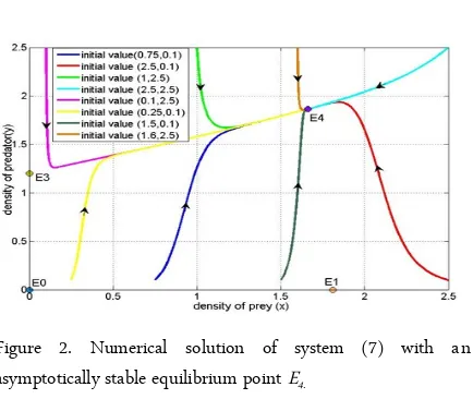
For the second simulation, we use the same parameter values as before except for parameter m1 and
m2. In this simulation, the values of m1 and m2 are
re-spectively 1.07 and 2. There are four equilibrium points i.e. E0 = (0,0), E1= (1.8101,0), E3 = (0,1.2) and E4 =
(1.66299,1.86519). The eigenvalues of J(E0) are 0.0196
and 0.2, the eigenvalues of J(E1) are -0.03754 and 0.2,
and the eigenvalues of J(E3) are -0.2 and -0.01736. On
the other hand, the eigenvalues of J(E4) are -0.03321
and -0.198827.
Therefore, E0, E1 and E3 are unstable and E4 is
asymptotically stable. In Figure 2, we plot some merical solutions using several initial values. All nu-merical solutions of system (7) converge to E4. Note
that in this simulation, we use greater values of m1 and
m2, meaning that the harvesting is decreased.
Conse-quently, prey can survive although the intrinsic growth rate of prey is low. The presence of food (prey) causes predator to survive. Therefore, predator and prey can coexist in the long term if prey harvesting is reduced.
In this paper, we have studied a modified Leslie-Gower predator-prey model with Beddington-DeAnge-lis functional response and MichaeBeddington-DeAnge-lis-Menten type prey harvesting numerically. It is found that the model has five equilibrium points (E0), namely the extinction of
both prey and predator point the predator extinction point (E and E), the prey extinction point (E), and
the survival of both prey and predator point (E4).
Based on numerical simulations, there are two possible stable equilibrium points that are E3 and E4. E3 and E4
respectively indicated the prey extinction or the survival both prey and predator in the long term. In the future, we will explore the dynamics of the model analytically.
1. Campbell NA, Reece JB, Mitchell LG (2004) Bi-ologi Vol. 3. 5th Ed. Erlangga. Jakarta.
2. Molles MC (2002) Ecology Concept and Applica-tions. 2nd Edition. Mc Graw Hill. Mexico City. 3. Holling CS (1965) The Functional Response of
Predator to Prey Density and its Role in Mimicry and Population Regulation. Memoirs of the Ento-mological Society of Canada. 97: 5-60.
4. Beddington JR (1975) Mutual Interference be-tween Parasites or Predators and its Effect on Searching Efficiency. Journal of Animal Ecology. 44: 331-340.
5. DeAngelis DL, Goldstein RA, O’Neill RV (1975) A Model of Trophic Interaction. Ecology. 56: 881-892.
6. Leslie PH (1948) Some Further Notes on the Use of Matrices in Population Mathematics. Biometrika. 35: 213-245.
7. Aziz-Alaoui MA, Okiye MD (2003) Boundedness and Global Stability for a Predator-Prey Model with Modified Leslie-Gower and Holling-type II schemes. Applied Mathemathics Letters. 16: 1069-1075.
9. Yu S (2014) Global Stability of a Modified Leslie-Gower Model with Beddington-DeAngelis Func-tional Response. Advances in Difference Equa