Case Study
Understanding hydrological
fl
ow paths in conceptual catchment
models using uncertainty and sensitivity analysis
Eva M. Mockler
a,n, Fiachra E. O
’
Loughlin
b, Michael Bruen
aaUCD Dooge Centre for Water Resources Research and UCD Earth Institute, University College Dublin, Dublin 4, Ireland
bSchool of Geographical Sciences, University of Bristol, Bristol BS8 1SS, United Kingdom
a r t i c l e
i n f o
Article history:
Received 16 February 2015 Received in revised form 27 August 2015 Accepted 31 August 2015 Available online 3 September 2015
Keywords:
Conceptual catchment modeling Hydrological processes Groundwater Sensitivity analysis Parameter identification
a b s t r a c t
Increasing pressures on water quality due to intensification of agriculture have raised demands for en-vironmental modeling to accurately simulate the movement of diffuse (nonpoint) nutrients in catch-ments. As hydrologicalflows drive the movement and attenuation of nutrients, individual hydrological processes in models should be adequately represented for water quality simulations to be meaningful. In particular, the relative contribution of groundwater and surface runoff to rivers is of interest, as in-creasing nitrate concentrations are linked to higher groundwater discharges. These requirements for hydrological modeling of groundwater contribution to rivers initiated this assessment of internalflow path partitioning in conceptual hydrological models.
In this study, a variance based sensitivity analysis method was used to investigate parameter sensitivities andflow partitioning of three conceptual hydrological models simulating 31 Irish catchments. We compared two established conceptual hydrological models (NAM and SMARG) and a new model (SMART), produced especially for water quality modeling. In addition to the criteria that assess streamflow simulations, a ratio of average groundwater contribution to total streamflow was calculated for all simulations over the 16 year study period. As observations time-series of groundwater contributions to streamflow are not available at catchment scale, the groundwater ratios were evaluated against average annual indices of baseflow and deep ground-waterflow for each catchment. The exploration of sensitivities of internalflow path partitioning was a specific focus to assist in evaluating model performances. Results highlight that model structure has a strong impact on simulated groundwaterflow paths. Sensitivity to the internal pathways in the models are not reflected in the performance criteria results. This demonstrates that simulated groundwater contribution should be constrained by independent data to ensure results within realistic bounds if such models are to be used in the broader environmental sustainability decision making context.
&2015 The Authors. Published by Elsevier Ltd. This is an open access article under the CC BY-NC-ND license (http://creativecommons.org/licenses/by-nc-nd/4.0/).
1. Introduction
In the natural environment, hydrological flows exist as a con-tinuum throughout the surface landscape and subsurface formations. Hydrological models attempt to capture the dominant processes in a catchment to predict river flows. For practical reasons, this flow continuum is simplified into discrete flow paths to facilitate con-ceptual understanding, model development and data analysis. The number of flow paths identified can depend on the catchment characteristics and the ultimate objective of the investigation, with two to fourflow paths typically representing responses offlow pro-cesses reaching a river (e.g. SMARG (Kachroo, 1992;Khan, 1986;Tan and O’Connor, 1996), HBV (Bergström, 1995), NAM (Nielsen and
Hansen, 1973)and PRMS (Leavesley et al., 1983,1996)).
The merits of conceptual, parametrically parsimonious, hydro-logical models for investigating the dominant pathways and pro-cesses in catchments have been widely discussed (e.g.Refsgaard and Henriksen, 2004;Sivapalan, 2003). Model parameter identi-fication is a fundamental challenge for hydrologists (Duan et al., 2006;Sivapalan, 2003). The presence of parameter interactions in conceptual rainfall–runoff (CRR) models can make a priori
para-meter prediction methods unreliable (Wagener and Wheater, 2006). Ideally, a model should be parametrically parsimonious while still capturing the dominant processes of the catchment with limited parameter interactions. Many hydrological models have been developed and used for decades for both research and operational hydrology. However, new model structures are still being developed to incorporate new conceptual understanding of specific catchment processes and places (Beven, 1999), and to fa-cilitate the demands of new pressures on water resources, in-cluding nutrient enrichment (Futter et al., 2014).
Contents lists available atScienceDirect
journal homepage:www.elsevier.com/locate/cageo
Computers & Geosciences
http://dx.doi.org/10.1016/j.cageo.2015.08.015
0098-3004/&2015 The Authors. Published by Elsevier Ltd. This is an open access article under the CC BY-NC-ND license (http://creativecommons.org/licenses/by-nc-nd/4.0/).
nCorresponding author.
There is a growing body of literature investigating model structure uncertainty (Breuer et al., 2009;Clark et al., 2008;Gupta et al., 2012;Kavetski and Fenicia, 2011;Wagener et al., 2001). The focus is increasingly turning to the internal movement of water within these conceptual models to investigate if each of the si-mulated processes contributing to the totalflows are realistic (e.g. Fenicia et al., 2011; Kokkonen and Jakeman, 2001). This hydro-logical partitioning is particularly important when couplingflow simulations with water quality, as theflow path can have a sig-nificant effect on solute transport and attenuation (Futter et al., 2014; Medici et al., 2012). Typically, particulate phosphorus is delivered via overlandflow (Jordan et al., 2005). Nitrate is typically delivered to streams via subsurface pathways, with links between increasing nitrate concentrations and groundwater contributions (Tesoriero et al., 2009).
Sensitivity analysis (SA) is “the principal evaluation tool for
characterizing the most and least important sources of uncertainty in environmental models” (U.S.EPA, 2009). The central role of sensitivity analysis for testing and implementing environmental models is widely noted (Refsgaard et al., 2007; U.S.EPA, 2009). Sensitivity analysis of parameters of water quality models has been undertaken using one-at-a time sensitivity analysis (e.g. Morris, 1991) with Latin Hypercube Sampling, for example, for simulating dissolved oxygen with the ESWAT model ( Vanden-berghe et al., 2001) and nitrogen with the INCA-N model ( Ranki-nen et al., 2013), or other Monte Carlo methods (e.g. McIntyre et al., 2005;Sánchez-Canales et al., 2015). More recently, variance
based sensitivity methods have been employed for the parameters of SWAT (Nossent et al., 2011;Zhang et al., 2013).
Variance based sensitivity analysis (e.g. Sobol, 2001) is re-commended as a superior method for which the computational effort is not prohibitive (Saltelli and Annoni, 2010; Tang et al., 2007; U.S.EPA, 2009). For non-linear conceptual hydrological models such as those investigated in this study, variance based methods are ideal to investigate the parameter sensitivities and interactions in the global parameter space (e.g.O’Loughlin et al.,
2013;van Werkhoven et al., 2008,2009;Zhan et al., 2013). The aim of the study was to identify a suitable hydrological model that can represent the internal flow paths in Irish catch-ments. In this paper, a new model that was developed with a focus on sub-surface flow paths, SMART, is compared with two well-established conceptual models, NAM and SMARG. The parameters and internalflow paths the three models are compared using (i) an uncertainty analysis and (ii) a variance based sensitivity analysis method. The analysis is carried out on multiple metrics of the three models simulating a 16 year period in 31 Irish catchments.
2. Data
2.1. Catchment data
The majority of Ireland's area (70,000 km2) has central, gently undulating lowlands of elevations generally less than 150 m above
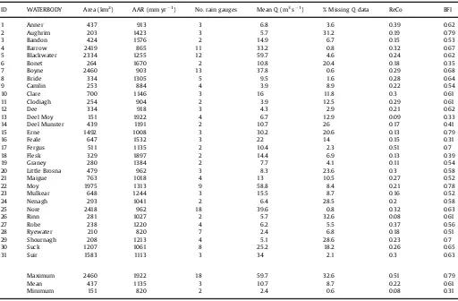
sea level, with areas of higher elevations near coasts. Annual rainfall varies from in excess of 3000 mm in the western moun-tains to less than 800 mm along the east coast. Mean annual temperatures range between 9°C and 10°C.
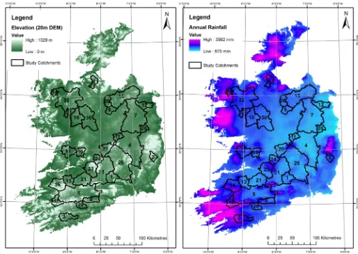
The 31 study catchments (Fig. 1,Table 1) were selected on the basis of having good quality meteorological and hydrometric data available for the 16 year study period beginning from 1 January 1990. The chosen catchments cover over 35% of the country and represent a variety of meteorological and geological conditions across Ireland, with catchment areas ranging from 151 km2 to 2460 km2.
Meteorological data consisted of daily rainfall and potential evapotranspiration values obtained from the Irish meteorology office, Met Éireann. The catchment-area averaged rainfall was calculated using the Thiessen method, with each catchment using data from at least two precipitation stations and the largest catchment (Boyne) containing 13 stations. Annual average rainfall (AAR) ranges from 820 mm in the Ryewater to 1897 mm in the Flesk with an overall average of 1189 mm. Potential evapo-transpiration was obtained from ten stations distributed over the study area, with data from the nearest station selected for each catchment and assumed to be spatially uniform.
Hydrometric data for each catchment consisted of daily mean flows originating from the Irish Office of Public Works (OPW) and the Irish Environmental Protection Agency (EPA). Periods within the 16 years of the study with missingflow data at the catchment outlet were not included in the analysis. Of the 31 catchments, four have missingflow data for over 25% of the study period, with the majority having less than 10% missing values (Table 1).
2.2. Catchment groundwaterflow indices
Groundwater is the part of the sub-surface water that is in the saturated zone, which typicallyflows through aquifers, although it can expand with increasing moisture conditions to includeflow through the subsoils and soils. Two indices representing ground-water flow are used in this study to indicate proportion of groundwater contributing to streamflow in catchments:
1. The groundwater recharge coefficient (ReCo) is calculated from the Geological Survey of Ireland (GSI) groundwater re-charge map (Hunter Williams et al., 2013), and does not incorporate any streamflow time-series. ReCo represents the deep groundwater resource in a catchment. The main hydro-geological properties used to generate the map were soil drainage properties, subsoil permeability and subsoil thick-ness. For example, groundwaterflow is predicted as low in areas overlain by thick, low permeability clay, and where low permeability aquifers are not able to accept percolating waters. ReCo is calculated as the predicted annual ground-water recharge (mm) as a percentage of the annual effective rainfall (mm).
2. The Base Flow Index (BFI) is a measure of the proportion of streamflow that is drawn from natural storages in the catch-ment. It was calculated from streamflow time-series by the Office of Public Works (OPW) using the 5-day minima method (Institute of Hydrology, 1980). BFI is greater than the recharge coefficient as it can includeflow through soils and subsoils.
Table 1
Catchment characteristics including annual average rainfall (AAR), mean discharge (Q), average groundwater recharge coefficient (ReCo) and baseflow index (BFI). ID WATERBODY Area (km2) AAR (mm yr 1) No. rain gauges Mean Q (m3s 1) % MissingQdata ReCo BFI
1 Anner 437 913 3 6.8 3.6 0.39 0.62
2 Aughrim 203 1423 3 5.7 31.2 0.19 0.79
3 Bandon 424 1576 2 14.9 6.7 0.15 0.53
4 Barrow 2419 865 11 33.2 0.8 0.32 0.67
5 Blackwater 2334 1255 12 59.7 4.6 0.24 0.62
6 Bonet 264 1670 2 10.8 20.4 0.18 0.35
7 Boyne 2460 903 13 37.8 0.6 0.29 0.68
8 Bride 334 1305 5 9.5 1.6 0.28 0.64
9 Camlin 253 884 4 3.9 8.9 0.22 0.54
10 Clare 700 1146 3 16 11.8 0.3 0.61
11 Clodiagh 254 904 2 3.9 12.5 0.29 0.61
12 Dee 334 918 3 4.3 2.9 0.21 0.62
13 Deel Moy 151 1922 4 6.7 12.9 0.09 0.33
14 Deel Munster 439 1191 2 10.7 26 0.17 0.41
15 Erne 1492 1008 3 30.2 20.6 0.13 0.79
16 Feale 647 1532 3 22 14 0.15 0.31
17 Fergus 511 1135 2 10.4 2.3 0.51 0.7
18 Flesk 329 1897 2 14.4 6.9 0.13 0.39
19 Graney 280 1384 2 7.7 4.1 0.11 0.54
20 Little Brosna 479 962 3 8.3 23.6 0.3 0.58
21 Maigue 763 1018 4 13 10.5 0.27 0.52
22 Moy 1975 1313 9 58.8 8.4 0.21 0.78
23 Mulkear 648 1244 3 15.5 8.7 0.16 0.52
24 Nenagh 293 1041 2 6.4 28.5 0.2 0.58
25 Nore 2418 962 18 39.6 0.8 0.32 0.63
26 Rinn 281 1027 2 5.7 32.6 0.08 0.61
27 Robe 238 1220 4 6.2 5.5 0.37 0.56
28 Ryewater 210 820 7 2.4 6.8 0.18 0.51
29 Shournagh 208 1213 4 5.1 28.6 0.23 0.7
30 Suck 1207 1061 8 25.2 18.2 0.26 0.65
31 Suir 1583 1113 3 34 2.1 0.3 0.63
Maximum 2460 1922 18 59.7 32.6 0.51 0.79
Mean 437 1135 3 10.7 8.7 0.22 0.61
3. Methods
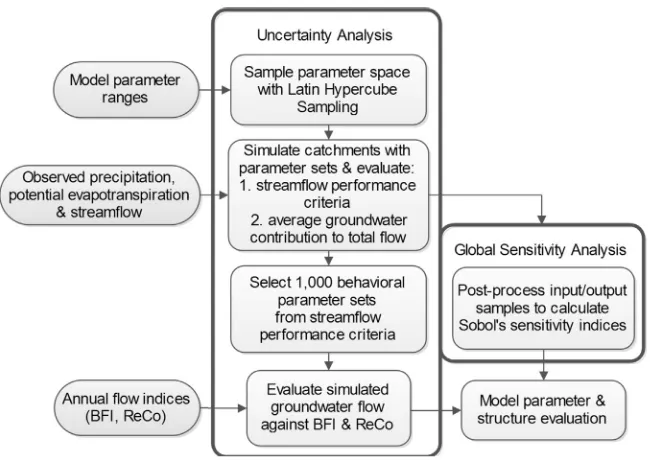
For three hydrological models, uncertainty and sensitivity analyses were undertaken on three model outputs (outlined in Section 3.2) generated from simulating each of the 31 catchments over the 16 year study period (Fig. 2).
3.1. Conceptual rainfall runoff models
Two established models (Sections 3.1.1and3.1.2), and a newly developed model (Section 3.1.3) were selected for this study. Fur-ther background information on hydrological models and appli-cations can be found in Singh and Frevert (2005) and Beven (2012).
3.1.1. NAM model
The‘Nedbør-Afstrømnings-Model’(NAM) model (Nielsen and
Hansen, 1973) is an internationally established model, and has previously been used in Irish catchments for investigating the contributions of groundwater and surface water to streamflow (Mockler and Bruen, 2013;O’Brien et al., 2013;RPS, 2008).
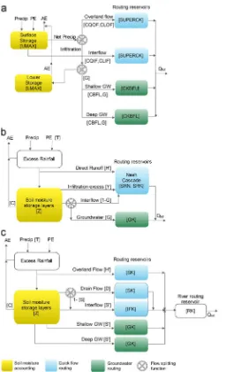
The NAM model has two storage reservoirs for soil moisture accounting and reservoirs representing four hydrological path-ways (Fig. 3a). Some small amendments were made to reduce the original 15-parameter NAM model to a more parsimonious 11-parameter structure. These included (i) omitting the snow com-ponent from the structure, as it is not relevant to the Irish study catchments, (ii) relating the two quickflow routing parameters of two linear reservoirs in series to one parameter (SUPERCK), and (iii)fixing the groundwater contribution factor equal to one (fol-lowing the assumption that groundwater transfers between catchments are negligible at this scale). Eight of these parameters control the moisture content in storages representing the surface, soil and groundwater storages, and three parameters relate to the routing components (Table 2a).
3.1.2. SMARG model
The Soil Moisture Accounting and Routing with Groundwater component (SMARG) model was developed in NUI Galway ( Ka-chroo, 1992;Khan, 1986;Tan and O’Connor, 1996). Its origins are in
the layers model (O’Connell et al., 1970) and its water balance
component is based on the ‘Layers Water Balance Model' (Nash
and Sutcliffe, 1970). The SMARG model has been widely applied in Irish catchments (Bastola et al., 2011; Goswami et al., 2005; O’Brien et al., 2013;RPS, 2008).
SMARG has a soil moisture accounting component that re-presents the catchment as a vertical stack of soil layers. This component keeps account of the rainfall, evaporation, runoff, and soil storage processes using six parameters (Fig. 3b, Table 2b). When there is rainfall in a time step, the excess rainfall is calcu-lated as the depth of water that exceeds potential evapo-transpiration. This depth of water is used to calculate surface runoff, which is the sum of (i) direct runoff, (ii) infiltration excess, and (iii) a portion of saturation excess. The remainder of the sa-turation excess contributes to the groundwater, as determined by the groundwater weighting parameter (G). The routing compo-nent uses linear reservoirs with three parameters (Table 2b) to simulate the attenuation effects of the catchment.
3.1.3. SMART model structure
The SMART model was developed to facilitate water quality modeling in Irish catchments, and was informed by the strengths of the NAM and SMARG models. The model has six soil layers of equal depth (Fig. 3c,Table 2c), similar to the SMARG, with six soil moisture accounting parameters. Drainflow is included as a se-parateflow path in the model, as this can be an important path-way for nutrients in agricultural catchments (e.g. Madison et al., 2014), and is related to soil moisture excess and the drain para-meter (S), which varies between 0 and 1. Interflow is a combina-tion of soil moisture excess and outflow from the soil layers, cal-culated using the soil outflow coefficient (D). Shallow and deep groundwater pathways are each calculated from individual out-flow equations, also related to the outflow coefficient (D) para-meter. Further details on the SMART model development are available inMockler et al. (2014).
3.2. Uncertainty analysis and evaluation criteria
A parameter uncertainty analysis was undertaken for each hydrological models using Latin Hypercube sampling of the ranges
outlined inTable 2a–c, assuming uniform probability distribution functions (see Fig. 2). In addition to analysis of the full set of sampled parameter sets, 1000 behavioral parameter sets were identified for each model based on the streamflow simulation performance. Similar Monte Carlo methods are frequently used to sample possible variations in inputs and parameters using as-sumed probability distribution functions e.g. the GLUE metho-dology (Beven and Binley, 1992).
In this study, we used two performance criteria to assess the adequacy of the simulation of total streamflow against the ob-served streamflow. The first is based on the Nash Sutcliffe effi -ciency (NSE) (Nash and Sutcliffe, 1970), a widely used goodness of fit measure based on the error variance defined as
Q Q
Q Q
NSE 1 t
n
t t
1 o, m,
2
t 1 n
o,t o
2
= − ∑ ( − )
∑ ( − ¯ )
=
=
whereQo,tis the observedflow for time-stept,Qm,tis the modeled flow at time-stept, Q¯o is the mean observedflow andn is the
length of the time series. A bounded version of the Nash–Sutcliffe
criterion (Mathevet et al., 2006) was calculated as
C2M=NSE/ 2( −NSE)
The C2Mcriterion varies between 1 andþ1 and is less
opti-mistic for positive values compared to NSE, thereby generating a less skewed distribution.
The second criteria used is the mean residual error criterion (MR), which calculates the difference between simulated and ob-servedflows in the overall water balance as
n Q Q
MR 1
t n
t t
1
o, m,
∑
= ( − )
=
where Qo,t is the observed flow for time-step t and Qm,t is the
modeledflow at time-stept. MR evaluates the overall water bal-ance, whereas the NSE focuses on the correlation of the time series.
In addition to the criteria that assess streamflow simulations, a ratio of average groundwater contribution (GWavg) to total stream-flow was calculated for all simulations over the study period, as
Q
GW n t GW
n t
n t n
t avg
1
1 m,
1
1 m,
= ∑ ( )
∑ ( )
=
=
3.3. Variance based global sensitivity analysis
Sobol's method (Sobol, 1993) is a global sensitivity analysis (GSA) which decomposes the output variance into relative con-tributions from input parameters and interactions (e.g.Shin et al., 2013;Tang et al., 2007;van Werkhoven et al., 2009). A sensitivity index (SI) representing the importance of the driving variablei(Xi) to the output (Y) can be defined as (Saltelli and Annoni, 2010)
where Var() and E() are variance and expectation functions
respectively. This is a measure of thefirst-order sensitivity indices (FSI) of each parameter on the model output, often referred to as
the main effect (Saltelli et al., 2008). The total-order sensitivity indices (TSI) represents the total effect of a parameter including interactions, and can be defined as (Saltelli and Annoni, 2010)
E Y X
where X~idenotes the matrix of all factors but Xi. For this study,
Saltelli's scheme [e.g. Saltelli et al., 2008, 2010] was used to compute FSI and TSI withn k( + )2 Monte Carlo simulations, where
kis the number of parameters andnis the initial sample size used (9000 in this study). This results in 99,000, 108,000 and 117,000 simulations for the 9, 10 and 11 parameter model, respectively. For each model, parameter sets were generated using Latin Hypercube sampling with uniform distributions following the ranges detailed in Table 2(a–c). Saltelli's scheme was computed using the SAFE
Toolbox (Pianosi et al., 2015)as a framework for assessment of the robustness and convergence of the sensitivity indices.
O’Loughlin et al. (2013) evaluated the parameters of the SMARG model with variance-based sensitivity analysis, and showed that sensitivities vary with time-step, flow regime and evaluation metric. In this study, all models use a daily time-step and are evaluated over the full range of flow regimes with the 16 year study period.
For the purpose of GSA, the GWavgratio was treated as a model output, with SI and TSI calculated in the same manner as the C2M and MR criteria. As observations time-series of groundwater con-tributions to streamflow are not available at catchment scale, the groundwater ratios were evaluated against average annual indices of base flow (BFI) and deep groundwater flow (ReCo) for each catchment (described inSection 2.2).
The sensitivity indices were compared to AAR to see if para-meters have a different importance based on hydrological regimes, as identified by AAR. The Spearman rank correlation coefficient (r)
was preferred over Person'sR2to assess the relationships between sensitivity indices and AAR as variables may be non-normally distributed and a linear relationship between the variables was not assumed.
4. Results and discussion
4.1. Uncertainty analysis and hydrological model performance
4.1.1. Hydrograph simulations
Results from the simulations using the Latin Hypercube sam-pling parameter sets show that for each catchment, each model had some simulations that performed well at simulating stream-flow, as evaluated by C2M(Fig. 4) and MR. The mean C2Mresults were 0.44, 0.18, 0.51 for the NAM, SMARG and SMART model, re-spectively, with results varying between catchments. The selection of parameter ranges (Table 2) and assumption of uniform dis-tributions between these ranges have an influence on these re-sults, and were guided by previous studies and literature.
Behavioral parameter sets were selected as the top 1000 for each hydrological model from equal weighting of C2Mand|MR|, as
evaluated against the observedflow data. The SMART model had the highest C2Mvalues, followed by the NAM and SMARG models (Table 3).
Sources of uncertainties in conceptual hydrological modeling results can arise in (i) model context, (ii) model structure, (iii) forcing data and (iv) parameters (Walker et al., 2003). The results presented in this paper assume that the model context is sound and do not include uncertainty due to observed rainfall, potential evapotranspiration and streamflow time-series, in order to facil-itate the focus on the model structure and internal flow partitioning.
Table 2a
NAM-based model parameter ranges for uncertainty and sensitivity analysis.
Parameter Description Range
UMAX Upper layer storage capacity (mm) 1.0–50.0 LMAX Lower layer storage capacity (mm) 20.0–500.0 CQOF Runoff coefficient in overlandflow equation 0.01–1.0 CLOF Threshold coefficient in overlandflow equation 0.0–0.8 CQIF Drainage coefficient in interflow equation (1/h) 0.00001–0.05 CLIF Threshold coefficient in interflow equation 0.0–0.95 CLG Threshold coefficient in recharge equation 0.0–0.95 CBFL Part of recharge going to lower groundwater 0.0–0.95 SUPERCK Time constant of linear reservoir for routing OF
and IF (h)
6.0–100.0
CKBFU Time constant of upper groundwater storage (h)
1000–4000
CKBFL Time constant of lower groundwater storage (h)
2000–8000
Table 2b
SMARG parameter ranges for uncertainty and sensitivity analysis.
Parameter Description Range
C Evaporation decay parameter 0.5–1
Z Combined water storage depth capacity of the layers (mm)
25–125
Y Maximum infiltration capacity depth (mm/time step)
10–100
H ‘Direct runoff' coefficient 0–1
T Evaporation parameter 0.5–1
G Groundwater weighting parameter 0–1 SRN Shape parameter of the Nash gamma
function quickflow routing
1–10
SRK Scale (lag) parameter of Nash gamma function quickflow routing (days)
1–20
GK Groundwater linear reservoir routing parameter (days)
1–200
Table 2c
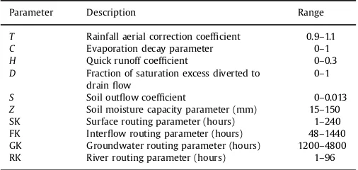
SMART parameter ranges for uncertainty and sensitivity analysis.
Parameter Description Range
T Rainfall aerial correction coefficient 0.9–1.1
C Evaporation decay parameter 0–1
H Quick runoff coefficient 0–0.3
D Fraction of saturation excess diverted to drainflow
0–1
4.1.2. Assessment of groundwater simulations
We further examined the 1000 behavioral simulations for each hydrological model, with a focus on groundwater contribution to streamflow. It is noteworthy that the behavioral sets were not selected using an objective function that optimizes groundwater simulations, such as the NSE with log values (Krause et al., 2005). Rather, this study aimed to assess the groundwater contribution of simulations that would be suitable for a range of low to highflows, as is required in catchment simulations for water quality (Futter et al., 2014;Medici et al., 2012). Moreover, the simulations were not constrained by the groundwater indices (BFI or ReCo) that were used in this assessment, and instead were used as in-dependent evaluators.
Fig. 5shows the distribution of GWavgby hydrological model for the 1000 behavioral sets, and for all model simulations using Latin Hypercube sampling. For each model, the distribution of GWavgfor the total number of sampling sets and the 1000 beha-vioral sets are broadly similar. These results highlight that the majority of NAM model simulations have a lower contribution of groundwater than is indicated by both the ReCo, which represents the deep groundwater, and the BFI, which represents total base flow contributions. The distributions of GWavgfor the SMARG and SMART models are more closely aligned with the ReCo and BFI values.
The internalflow partitioning for each catchment was notably different across the models. To demonstrate this, the percentage of groundwater contributing to simulated streamflow was compared with catchment groundwaterflow indices. Correlations between GWavg results and the BFI and ReCo (defined inSection 2.2) in-dicate whether the internal hydrological processes of the models are aligned with the understanding of processes from catchment
characteristics. Of the three models, the SMART model had the strongest correlations with ReCo and BFI values across the catch-ments (Table 3). This indicates that the processes of SMART that produce quick in-stream responses and groundwater flow are more representative of what is expected from catchment characteristics.
The range of simulated GWavgfor each catchment produced by the 1,000 simulations indicated the degree of uncertainty in at-tributingflow to quickflow or groundwater. The SMARG had the widest prediction ranges, which tended to increase with increas-ing BFI (Fig. 8) i.e. greater uncertainty in groundwater dominated catchments. The SMART model produced tighter ranges of GWavg estimates (Table 3,Fig. 6), indicating that the SMART model has less uncertainty simulating internal processes, without providing any additional groundwater or baseflow information.
There is a growing body of literature highlighting the im-portance of assessing model structure adequacy (Breuer et al., 2009;Clark et al., 2008;Gupta et al., 2012;Wagener et al., 2001). In this study, the three conceptual models have different re-presentations of surface runoff (or quickflow) and groundwater contributions to streamflow. All three models assume that the surface water and groundwater of the study catchments aligned, and that there are no transfers into or out of the catchment. This assumption may not be true, particularly for catchments with extensive subsurface paleochannels crossing catchment bound-aries, or conduit karst aquifers i.e. Clare, Fergus, Robe and Suck catchments. The NAM and SMART models have more detailed internal flow partitioning compared to the SMARG model, and therefore are lessflexible to adapt to different hydrological con-ditions. In particular, the internalflow paths of catchments with conduit karst aquifer bedrock may need to be interpreted, where a
simulated quick flow path is actually representing the ground-water conduitflow.
4.2. Global sensitivity analysis
Assessing the convergence and uncertainty bounds (from bootstrap sampling) of the sensitivity indices identified the base
sample size for Latin Hypercube sampling. Although convergence of SI and TSI was achieved for all models for the C2Mand MR model output with a base sample of 5000, the SI and TSI values for GWavg output required an increased base sample size (9000) to achieve convergence. The base sample size of 9000 was selected which produced relatively tight uncertainty bounds (average TSI confidence intervals between 0.04 and 0.12) for the streamflow
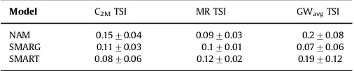
Table 3
Summary of C2M, MR and GWavgresults for the 31 catchments and correlation of GWavgwith catchment recharge coefficients (ReCo) and baseflow indices (BFI) for 1000
behavioral simulations for 3 models.
Model C2Mmedian (min, max) MR median (min, max) Gwavgmedian (min, max) GWavgcorr with ReCo GWavgcorr with BFI
NAM 0.6 (0.34,0.84) 0.01 ( 0.19,0.2) 0.12 (0,0.87) 0.18 (p¼0.32) 0 (p¼0.98) SMARG 0.59 (0.21,0.9) 0 ( 0.32,0.19) 0.33 (0,0.99) 0.37 (p¼0.04) 0.66 (pr0.01) SMART 0.65 (0.39,0.85) 0 ( 0.17,0.08) 0.42 (0,0.7) 0.45 (p¼0.01) 0.87 (pr0.01)
Fig. 5.Distribution of the fraction of groundwater contributing to totalflow for 31 catchments from NAM (blue), SMARG (yellow) and SMART (red) for all model simulations (‘all'; dashed line) and behavioral sets (‘best'; solid line) using Latin Hypercube sampling of standard parameter ranges with uniform distributions. (For interpretation of the references to color in thisfigure legend, the reader is referred to the web version of this article.)
0.0 0.2 0.4 0.6 0.8
NAM Simulated GWavg SMARG Simulated GWavg
0.0 0.2 0.4 0.6 0.8 0.0 0.2 0.4 0.6 0.8 0.0 0.2 0.4 0.6 0.8 SMART Simulated GWavg
SMART SMARG NAM
Catchment BFI
Fig. 6.Simulated groundwater contribution (GWavg) against BFI for each study catchment for the NAM (blue), SMARG (orange) and SMART (red) models. (For interpretation
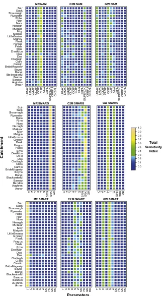
performance criteria (C2Mand MR), as indicated by the standard deviation results from bootstrap sampling (Table 4). This is in line with average TSI confidence intervals values reported in similar studies e.g. Tang et al. (2007) (values between 0.0 and 0.12 for daily time-step) and (Nossent et al., 2011) (values between 0.1 and 0.14). The uncertainty ranges for GWavgindices were wider (twice the standard deviation for C2M, seeTable 4), therefore the rank of sensitive parameters are uncertain. Nonetheless, the sensitive parameters were still clearly identifiable from the results (Fig. 7) and this was deemed sufficient for a general parameter assess-ment to support the uncertainty analysis.
In the following sections, long-term average Sobol's sensitivity results from the 16 year study period are presented for each model in turn.Fig. 7shows the TSI for all model parameters across the 31 study catchments in color-coded grids with blue indicating low values (o0.1) and orange indicating high values (40.8). Some TSI
had slightly negative values, particularly with C2Mmodel output, which were attributed to numerical errors in the Saltelli method. As these occur for sensitivity indices when the analytical sensi-tivity indices are close to zero, only unimportant factors are af-fected (Saltelli et al., 2008). Changes in the sampling ranges of sensitive parameters can impact sensitivity results (Shin et al., 2013). In order to ensure comparable results across catchments in this study, broad parameter ranges that include suitable values for all study catchments were selected.
van Werkhoven et al. (2008)used Sobol's sensitivity analysis to assess the parameters of a conceptual rainfall–runoff model across
a hydroclimatic gradient with a narrower range of AAR compared to those of this study, but a wider range of annual potential eva-potranspiration. Similar to results from that study,Fig. 7 shows that, across all of the models, less parameters have notable SI values for the long term average model output (MR), compared to the peak-fitting evaluation criteria (C2M). Similar to findings of Zhan et al. (2013), routing parameters of the NAM (SUPERCK), SMARG (SRK) and SMART (SK) models are sensitive when eval-uated by NSE based output (C2Mresults;Fig. 7)
4.2.1. NAM sensitivity results
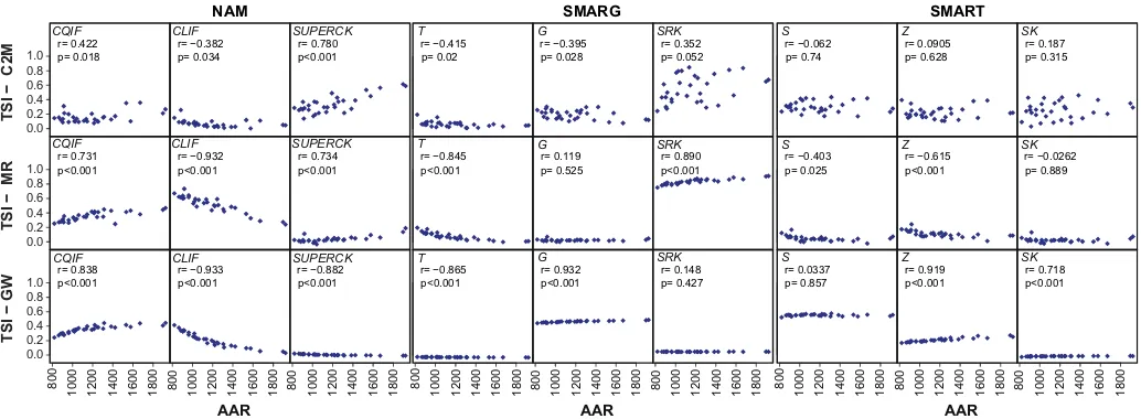
The interflow threshold coefficient (CLIF) is the predominantly sensitive parameter in the NAM model in relation to the overall water balance, reflected in results from the MR output. CLIF affects the water volume available to satisfy evapotranspiration demands in NAM's lower storage when demands that cannot be met by the upper storage, and thus the water balance. Sensitivity indices for CLIF increases with decreasing values of catchment AAR (r¼ 0.93,po0.001;Fig. 8). Moderate sensitivity indices are also identified for the interflow coefficient (CQIF), which tend to in-crease as catchment AAR inin-creases (r¼0.73,po0.001;Fig. 8) and are strongly negatively correlated (r¼ 0.9, po0.001) with the threshold coefficient (CLIF). Thus, CLIF is more identifiable in drier catchments where the volume in the lower store is more variable. In catchments with relatively high annual average rainfall, the lower store remains full and thus unchanging, for long periods, resulting in the interflow coefficient (CQIF) being relatively more sensitive.
The quickflow routing parameter (SUPERCK) is the most sen-sitive parameter when evaluated with C2M. Correlations between TSI and catchment AAR (r¼0.78,po0.001;Fig. 8), suggest that the SUPERCK parameter is more identifiable in wetter catchments. Contrasting trends are evident between first-order and higher-order indices for SUPERCK, indicating that when the parameter is identifiable, parameter interactions are reduced.
The highest TSIs for NAM's GWavg output are the upper layer storage capacity (UMAX) and the interflow coefficient (CQIF). CQIF has prominent sensitivities for the groundwaterflow processes, even though this parameter is not directly in the process equa-tions. This is because all of the internalflow paths in the NAM model, including groundwater, areproportional to the relative volume in the lower zone store, which is related to the interflow parameters (CQIF and CLIF). Therefore, the interflow parameters are sensitive with respect to many of the internal processes in NAM (Fig. 7). This soil moisture accounting mechanism does not represent the natural draining mechanisms in catchment, as the lower zone store can only be depleted by evapotranspiration.
4.2.2. SMARG sensitivity results
The quick flow routing lag parameter of the Nash gamma function (SRK) is the most sensitive when evaluated by the C2M and MR criteria. When evaluated by MR, the SRK sensitivities are due to the curtailment of the unit pulse response function when inappropriate parameter values are selected during optimization (Goswami and O’Connor, 2010). The sensitivities only relate to
high flows (as seen in O’Loughlin et al., 2013), and are present across all catchments, regardless of appropriate impulse response function memory length. TSI values for SRK have positive corre-lations with AAR for MR output (r¼0.89, po0.001;Fig. 8), in-dicating that the routing lag parameter is more sensitive in wetter catchments. An opposing trend is seen for TSI values for the eva-potranspiration coefficient (T) which is an adjustment factor for potential evapotranspiration input data, as the T parameter is
more sensitive in drier catchments. The maximum infiltration capacity parameter (Y) and evaporation decay parameter (C) are not sensitive for any of the three criteria (also seen inO’Loughlin et al., 2013). The soil layer depth parameter (Z) also shows very low SI values across all the study catchments. This is due to the structure of equations of the SMARG model, and may result in difficulty identifying parameter values, particularly for temperate climate conditions such as Ireland.
The‘direct runoff' coefficient (H) and groundwater weighting parameter (G) are prominent in the groundwaterflow evaluation (GWavg), as these parameters determine the internal split offlows in the model. They are not notable in the evaluation by model performance (C2Mand MR) as these are calculated on totalflows.
4.2.3. SMART sensitivity results
For the SMART model, the catchment rainfall correction coef-ficient (T) consistently shows high TSI values for the MR output as this parameter adjusts the precipitation input to match the ob-servedflows. The impact of this parameter increases as the volume of precipitation increases, with TSI values positively correlated with AAR (r¼0.87,po0.01;Fig. 8).
Trends in values of TSI are less defined for C2M evaluation, compared to MR, with moderate values for the soil moisture outflow parameter (S) and soil moisture capacity parameter (Z). As subsurfaceflow partitioning is determined from drainage calcu-lated from the soil moisture storage layers, theSandZhave high
TSI values across all catchment when evaluated by the GWavg output.
The SMART model was developed with a focus on sub-surface flow paths, driven by challenges of simulating diffuse nutrient impacts on water quality. As the model development was
Table 4
Mean and standard deviation (from bootstrapping) of total-order sensitivity indices (TSI) across all parameters as evaluated by mean residual (MR), bounded NSE (C2M)
and average groundwater fraction (GWavg) model output for the NAM, SMARG and
SMART.
Model C2MTSI MR TSI GWavgTSI
NAM 0.1570.04 0.0970.03 0.270.08
SMARG 0.1170.03 0.170.01 0.0770.06
informed from components of the NAM and SMARG models, a comparison of model structures is of interest. The SMART model structure was designed on the concept of the SMARG soil moisture layers, with the following notable changes;
1. The maximum infiltration capacity parameter (Y) of the SMARG
was not included in the SMART model as it is a difficult para-meter to estimate at catchment scale. Instead, the infiltration excess process was conceptually combined with‘direct' runoff.
2. The evaporation coefficient (C) and soil moisture capacity
parameter (Z) of the SMARG model showed very lowfirst order sensitivities (both with an average TSI of 0 for all evaluation
MR NAM
UMAX LMAX CQOF CLOF CQIF CLIF CLG CBFL
SUPERCK
UMAX LMAX CQOF CLOF CQIF CLIF CLG CBFL
SUPERCK
CKBFU CKBFL UMAX LMAX CQOF CLOF CQIF CLIF CLG CBFL
Fig. 7.Total-order sensitivity indices (TSI) evaluated by mean residual (MR), bounded NSE (C2M) and average groundwater fraction (GWavg) model output for the NAM (top
criteria), indicating poorly identifiable parameters. The SMART model structure incorporates the soil moisture layer concept of the SMARG model, but the structural changes included re-defining the soil layers and outflows. This resulted in increases in TSI for theZparameter from an average of 0 in the SMARG model to 0.18 in the SMART (Fig. 7: SMART results). As evaporation is calculated from the soil layers, there was also an increase in average catchment TSI for theCparameter for MR from 0 in the SMARG model to 0.12 (Fig. 7: MR SMART results). 3. Linear reservoirs were selected for routing quickflow, similar to the NAM model, in place of the Nash cascade routing compo-nent of the SMARG model. This resulted in reduced parameter interactions and the conservation of volume in the routing component of the SMART model.
5. Conclusions
For coupled water quantity and water quality modeling, a hy-drological model is required that can capture both the totalflows and the groundwater contributions to streamflow. A comparison of results from Monte Carlo simulations of 31 study catchments for the NAM, SMARG and SMART models highlight that the relative contribution of groundwater depends on both the model structure and the catchment characteristics. Results showed that the new SMART model was superior to the two established models, NAM and SMARG, at representing both the total streamflow and the internalflow paths of the 31 Irish study catchments.
The SMART model development was influenced by the favor-able aspects of the SMARG and NAM structures to enhance model parameter identification while maintaining a structure that can properly identify overland, interflow, upper and lower ground-waterflow as discreteflow paths contributing to streamflow. Re-sults from Sobol's sensitivity method confirmed that the SMART model development reduced the number of poorly identifiable parameters, compared to the SMARG model.
Internalflow partitioning varies greatly between models and, to varying degrees, between behavioral parameter sets for each model. This study illustrated this by comparing the simulated annual groundwater contributions to streamflow with additional independent information, in the form of groundwaterflow indices. For studies interested coupling water quality and hydrological si-mulations, it is recommended that an appropriate model structure is selected and, where available, additional information on
plausible groundwater flow contributions is incorporated into model calibration.
Acknowledgments
The data for this paper are available from Met Eireann, OPW, and the Irish EPA. This work was supported by the Environmental Pro-tection Agency Research Programme through the STRIVEPathways
Project(2007-WQ-CD-1-S1) and theCatchmentTools Project
(2013-W-FS-14). Dr Fiachra O'Loughlin is funded by the Leverhulme Trust (RPG-409). The authors would like to thank B.Elsasser for providing data for this research. We are particularly gratefully to the anonymous re-viewers who considerably helped in improving the manuscript.
References
Bastola, S., Murphy, C., Sweeney, J., 2011. Evaluation of the transferability of hy-drological model parameters for simulations under changed climatic condi-tions. Hydrol. Earth Syst. Sci. Discuss. 8, 5891–5915.http://dx.doi.org/10.5194/ hessd-8-5891-2011.
Bergström, S., 1995. The HBV Model. Water Resources Publications, Colorado, pp. 443–476.
Beven, K., 2012. Down to Basics: Runoff Processes and the Modelling Process. In: Rainfall–Runoff Modelling. John Wiley & Sons, Ltd. pp. 1–23.
Beven, K., Binley, A., 1992. The future of distributed models—model calibration and uncertainty prediction. Hydrol. Process. 6 (3), 279–298.http://dx.doi.org/ 10.1002/hyp.3360060305.
Beven, K.J., 1999. Uniqueness of place and process representations in hydrological modelling. Hydrol. Earth Syst. Sci. 4 (2), 203–213.http://dx.doi.org/10.5194/ hess-4-203-2000.
Breuer, L., et al., 2009. Assessing the impact of land use change on hydrology by ensemble modeling (LUCHEM). I: model intercomparison with current land use. Adv. Water Resour.32(2), 129–146.http://dx.doi.org/10.1016/j. advwatres.2008.10.003.
Clark, M.P., Slater, A.G., Rupp, D.E., Woods, R.A., Vrugt, J.A., Gupta, H.V., Wagener, T., Hay, L.E., 2008. Framework for Understanding Structural Errors (FUSE): a modular framework to diagnose differences between hydrological models. Water Resour. Res. 44 (12), W00B02.http://dx.doi.org/10.1029/2007wr006735. Duan, Q., et al., 2006. Model Parameter Estimation Experiment (MOPEX): an
overview of science strategy and major results from the second and third workshops. J. Hydrol. 320 (1–2), 3–17.http://dx.doi.org/10.1016/j. jhydrol.2005.07.031.
Fenicia, F., Kavetski, D., Savenije, H.H.G., 2011. Elements of aflexible approach for conceptual hydrological modeling: 1. Motivation and theoretical development. Water Resour. Res. 47. http://dx.doi.org/10.1029/2010wr010174.
Futter, M.N., Erlandsson, M.A., Butterfield, D., Whitehead, P.G., Oni, S.K., Wade, A.J., 2014. PERSiST: aflexible rainfall–runoff modelling toolkit for use with the INCA family of models. Hydrol. Earth Syst. Sci.18(2), 855–873.http://dx.doi.org/ 10.5194/hess-18-855-2014.
Goswami, M., O’Connor, K.M., 2010. A“monster”that made the SMAR conceptual
CQIF
1000 1200 1400 1600 1800 0.0
800 1000 1200 1400 1600 1800
r= −0.882 p<0.001
800 1000 1200 1400 1600 1800
AAR
1000 1200 1400 1600 1800 800 1000 1200 1400 1600 1800 800 1000 1200 1400 1600 1800
AAR
800
1000 1200 1400 1600 1800 800 1000 1200 1400 1600 1800 800 1000 1200 1400 1600 1800
AAR
model“right for the wrong reasons”. Hydrol. Sci. J. 55 (6), 913–927.http://dx. doi.org/10.1080/02626667.2010.505170.
Goswami, M., O’Connor, K.M., Bhattarai, K.P., Shamseldin, A.Y., 2005. Assessing the performance of eight real-time updating models and procedures for the Brosna River. Hydrol. Earth Syst. Sci. 9 (4), 394–411.http://dx.doi.org/10.5194/ hess-9-394-2005.
Gupta, H.V., Clark, M.P., Vrugt, J.A., Abramowitz, G., Ye, M., 2012. Towards a com-prehensive assessment of model structural adequacy. Water Resour. Res. 48 (8). http://dx.doi.org/10.1029/2011WR011044.
Hunter Williams, N.H., Misstear, B.D.R., Daly, D., Lee, M., 2013. Development of a national groundwater recharge map for the Republic of Ireland. Q. J. Eng. Geol. Hydrogeol. 46 (4), 493–506.http://dx.doi.org/10.1144/qjegh2012-016. Institute of Hydrology, 1980. Low Flow Studies Research Report. Wallingford, U.K. Jordan, P., Menary, W., Daly, K., Kiely, G., Morgan, G., Byrne, P., Moles, R., 2005.
Patterns and processes of phosphorus transfer from Irish grassland soils to rivers—integration of laboratory and catchment studies. J. Hydrol. 304 (1–4), 20–34.http://dx.doi.org/10.1016/j.jhydrol.2004.07.021.
Kachroo, R.K., 1992. Riverflow forecasting. 5. Applications of a conceptual-model. J. Hydrol. 133 (1–2), 141–178.http://dx.doi.org/10.1016/0022-1694(92)90150-T. Kavetski, D., Fenicia, F., 2011. Elements of aflexible approach for conceptual hy-drological modeling: 2. Application and experimental insights. Water Resour. Res. 47. http://dx.doi.org/10.1029/2011wr010748.
Khan, H., 1986. Conceptual Modelling of Rainfall–runoff Systems, National Uni-versity of Ireland, Galway.
Kokkonen, T.S., Jakeman, A.J., 2001. A comparison of metric and conceptual ap-proaches in rainfall–runoff modeling and its implications. Water Resour. Res. 37 (9), 2345–2352.http://dx.doi.org/10.1029/2001WR000299.
Krause, P., Boyle, D.P., Bäse, F., 2005. Comparison of different efficiency criteria for hydrological model assessment. Adv. Geosci.5, 89–97.http://dx.doi.org/ 10.5194/adgeo-5-89-2005.
Leavesley, G., Restrepo, P., Markstrom, S., Dixon, M., Stannard, L., 1996. The Modular Modeling System (MMS): User’s Manual. US Geol. Surv. Open File Rep. 96 (151), 142.
Leavesley, G.H., Lichty, R.,Troutman, B., Saindon, L., 1983. Precipitation-runoff Modeling System: User’s Manual. US Geological Survey.
Madison, A.M., Ruark, M.D., Stuntebeck, T.D., Komiskey, M.J., Good, L.W., Drummy, N., Cooley, E.T., 2014. Characterizing phosphorus dynamics in tile-drained agriculturalfields of eastern Wisconsin. J. Hydrol. 519 (0), 892–901.http://dx. doi.org/10.1016/j.jhydrol.2014.08.016Part A.
Mathevet, T., Michel, C., Andreassian, V., Perrin, C., 2006. A bounded version of the Nash–Sutcliffe criterion for better model assessment on large sets of basins. vol.
307. IAHS Publication, p. 211.
McIntyre, N., Jackson, B., Wade, A.J., Butterfield, D., Wheater, H.S., 2005. Sensitivity analysis of a catchment-scale nitrogen model. J. Hydrol. 315 (1–4), 71–92.http: //dx.doi.org/10.1016/j.jhydrol.2005.04.010.
Medici, C., Wade, A.J., Frances, F., 2012. Does increased hydrochemical model complexity decrease robustness? J. Hydrol. 440, 1–13.http://dx.doi.org/ 10.1016/j.jhydro1.2012.02.047.
Mockler, E., Bruen, M., Desta, M., Misstear, B., 2014. Pathways Project Final Report Volume 4: Catchment Modelling Tool (STRIVE Report). Environmental Protec-tion Agency, Ireland.〈http://erc.epa.ie/safer/iso19115/displayISO19115.jsp?iso ID¼196#files〉, p. 173.
Mockler, E.M., Bruen, M., 2013. Parameterizing dynamic water quality models in ungauged basins: issues and solutions. Underst. Freshw. Qual. Problems in a Chang. World361, 235–242.
Morris, M.D., 1991. Factorial sampling plans for preliminary computational ex-periments. Technometrics 33 (2), 161–174.http://dx.doi.org/10.2307/1269043. Nash, J.E., Sutcliffe, J.V., 1970. Riverflow forecasting through conceptual models
part I-A discussion of principles. J. Hydrol. 10 (3), 282–290.http://dx.doi.org/ 10.1016/0022-1694(70)90255-6.
Nielsen, S.A., Hansen, E., 1973. Numerical simulation of the rainfall–runoff process on a daily basis. Nord. Hydrol. 4, 171–190.http://dx.doi.org/10.2166/nh.1973.013. Nossent, J., Elsen, P., Bauwens, W., 2011. Sobol’sensitivity analysis of a complex
environmental model. Environ. Model. Softw. 26 (12), 1515–1525.http://dx.doi. org/10.1016/j.envsoft.2011.08.010.
O’Brien, R.J., Misstear, B.D., Gill, L.W., Deakin, J.L., Flynn, R., 2013. Developing an integrated hydrograph separation and lumped modelling approach to quanti-fying hydrological pathways in Irish river catchments. J. Hydrol. 486, 259–270. http://dx.doi.org/10.1016/j.jhydrol.2013.01.034.
O’Connell, P.E., Nash, J.E., Farrell, J.P., 1970. Riverflow forecasting through con-ceptual models Part II—the Brosna catchment at Ferbane. J Hydrol 10 (4), 317–329.http://dx.doi.org/10.1016/0022-1694(70)90221-0.
O’Loughlin, F., Bruen, M., Wagener, T., 2013. Parameter sensitivity of a watershed-scaleflood forecasting model as a function of modelling time-step. Hydrol. Res. 44 (2), 334–350.http://dx.doi.org/10.2166/Nh.2012.157.
Pianosi, F., Sarrazin, F., Wagener, T., 2015. A Matlab toolbox for Global Sensitivity Analysis. Environ. Model. Softw. 70 (0), 80–85.http://dx.doi.org/10.1016/j. envsoft.2015.04.009.
Rankinen, K., Granlund, K., Futter, M.N., Butterfield, D., Wade, A.J., Skeffington, R.,
Arvola, L., Veijalainen, N., Huttunen, I., Lepisto, A., 2013. Controls on inorganic nitrogen leaching from Finnish catchments assessed using a sensitivity and uncertainty analysis of the INCA-N model. Boreal Environ. Res. 18 (5), 373–386. Refsgaard, J.C., Henriksen, H.J., 2004. Modelling guidelines––terminology and
guiding principles. Adv. Water Resour. 27 (1), 71–82.http://dx.doi.org/10.1016/j. advwatres.2003.08.006.
Refsgaard, J.C., van der Sluijs, J.P., Højberg, A.L., Vanrolleghem, P.A., 2007. Un-certainty in the environmental modelling process–a framework and guidance. Environ. Model. Software22(11), 1543–1556.http://dx.doi.org/10.1016/j. envsoft.2007.02.004.
RPS, 2008. Further characterisation study: An integrated approach to quantifying groundwater and surface water contributions of streamflowRep., South-western River Basin District, Ireland.
Saltelli, A., Annoni, P., 2010. How to avoid a perfunctory sensitivity analysis. En-viron. Model. Softw. 25 (12), 1508–1517.http://dx.doi.org/10.1016/j. envsoft.2010.04.012.
Saltelli, A., Annoni, P., Azzini, I., Campolongo, F., Ratto, M., Tarantola, S., 2010. Var-iance based sensitivity analysis of model output. Design and estimator for the total sensitivity index. Comput. Phys. Commun. 181 (2), 259–270.
Saltelli, A., Ratto, M., Andres, T., Campolongo, F., Cariboni, J., Gatelli, D., Saisana, M., Tarantola, S., 2008. Global Sensitivity Analysis: The Primer. John Wiley & Sons. Sánchez-Canales, M., López-Benito, A., Acuña, V., Ziv, G., Hamel, P., Chaplin-Kramer, R., Elorza, F.J., 2015. Sensitivity analysis of a sediment dynamics model applied in a Mediterranean river basin: global change and management implications. Sci. Total Environ. 502 (0), 602–610.http://dx.doi.org/10.1016/j.
scitotenv.2014.09.074.
Shin, M.-J., Guillaume, J.H.A., Croke, B.F.W., Jakeman, A.J., 2013. Addressing ten questions about conceptual rainfall–runoff models with global sensitivity analyses in R. J. Hydrol. 503 (0), 135–152.http://dx.doi.org/10.1016/j. jhydrol.2013.08.047.
Singh, V.P., Frevert, D.K., 2005. Watershed Models. CRC Press.
Sivapalan, M., 2003. Prediction in ungauged basins: a grand challenge for theore-tical hydrology. Hydrol. Process. 17 (15), 3163–3170.http://dx.doi.org/10.1002/ hyp.5155.
Sobol, I.M., 1993. Sensitivity analysis for non-linear mathematical models. Math. Model. Comput. Exp. 1, 407–414.
Sobol, I.M., 2001. Global sensitivity indices for nonlinear mathematical models and their Monte Carlo estimates. Math. Comput. Simulat. 55 (1–3), 271–280.http: //dx.doi.org/10.1016/S0378-4754(00)00270-6.
Tan, B.Q., O’Connor, K.M., 1996. Application of an empirical infiltration equation in the SMAR conceptual model. J. Hydrol. 185 (1–4), 275–295.http://dx.doi.org/ 10.1016/0022-1694(95)02993-1.
Tang, Y., Reed, P., Wagener, T., van Werkhoven, K., 2007. Comparing sensitivity analysis methods to advance lumped watershed model identification and evaluation. Hydrol. Earth Syst. Sci. 11 (2), 793–817.http://dx.doi.org/10.5194/ hess-11-793-2007.
Tesoriero, A.J., Duff, J.H., Wolock, D.M., Spahr, N.E., Almendinger, J.E., 2009. Iden-tifying pathways and processes affecting nitrate and orthophosphate inputs to streams in agricultural watersheds. J. Environ. Qual. 38 (5), 1892–1900.http: //dx.doi.org/10.2134/jeq2008.0484.
U.S.EPA, 2009. Guidance on the Development, Evaluation, and Application of En-vironmental Models. Technical Report EPA/100/K-09/003Rep. Office of the Science Advisor, Council for Regulatory Environmental Modeling. 26 pp. van Werkhoven, K., Wagener, T., Reed, P., Tang, Y., 2008. Characterization of
wa-tershed model behavior across a hydroclimatic gradient. Water Resour. Res. 44 (1), W01429.http://dx.doi.org/10.1029/2007wr006271.
van Werkhoven, K., Wagener, T., Reed, P., Tang, Y., 2009. Sensitivity-guided reduc-tion of parametric dimensionality for multi-objective calibrareduc-tion of watershed models. Adv. Water Resour. 32 (8), 1154–1169.http://dx.doi.org/10.1016/j. advwatres.2009.03.002.
Vandenberghe, V., van Griensven, A., Bauwens, W., 2001. Sensitivity analysis and calibration of the parameters of ESWAT: application to the River Dender. Water Sci. Technol.43(7), 295–300.
Wagener, T., Wheater, H.S., 2006. Parameter estimation and regionalization for continuous rainfall–runoff models including uncertainty. J. Hydrol. 320 (1–2), 132–154.http://dx.doi.org/10.1016/j.jhydrol.2005.07.015.
Wagener, T., Boyle, D.P., Lees, M.J., Wheater, H.S., Gupta, H.V., Sorooshian, S., 2001. A framework for development and application of hydrological models. Hydrol. Earth Syst. Sci.5(1), 13–26.http://dx.doi.org/10.5194/hess-5-13-2001. Walker, W.E., Harremoës, P., Rotmans, J., van der Sluijs, J.P., van Asselt, M.B.A.,
Janssen, P., Krayer von Krauss, M.P., 2003. Defining uncertainty. A conceptual basis for uncertainty management in model-based decision support. Integr. Assess. 4 (1), 5–17.http://dx.doi.org/10.1076/iaij.4.1.5.16466.
Zhan, C.-s, Song, X.-m, Xia, J., Tong, C., 2013. An efficient integrated approach for global sensitivity analysis of hydrological model parameters. Environ. Model. Softw. 41 (0), 39–52.http://dx.doi.org/10.1016/j.envsoft.2012.10.009. Zhang, C., Chu, J., Fu, G., 2013. Sobol's sensitivity analysis for a distributed