http://iste.co.uk/index.php?f=x&ACTION=View&id=376>ȝȝ@
Publication Date: November 2010 Hardback 352 pp. 95.00 USD
Description
The surge, over the past few decades, in the application of computer-based information technologies has brought about the development of spatial analysis, GIS, and tools simulation that allow for the design of integrated, disaggregate-level models of urban dynamics.
The field of Urban Dynamics itself is based on the systems engineering concept that all complex systems (and cities and urban areas are no exception) are comprised of independent and often smaller, more understandable sub-components with relationships to one another. This allows for the system as a whole to be modeled, using knowledge of the individual subsystems and their behaviors. In this instance, urban dynamics allows for the modeling and understanding of land use, the attractiveness of space to residents, and how the ageing and obsolescence of buildings affects planning and economic development, as well as population movements, with the urban landscape.
The book adopts a trans-disciplinary approach that looks at the way residential mobility, commuting patterns, and travel behavior affect the urban form. It addresses a series of issues dealing with the accessibility of urban amenities, quality of life, and assessment of landscape residential choices, as well as measurement of external factors in the urban environment and their impact on property values.
Contents
1. The Role of Mobility in the Building of Metropolitan Polycentrism, Sandrine Berroir, Hélène Mathian, Thérèse Saint-Julien and Lena Sanders.
2. Commuting and Gender: Two Cities, One Reality?,Marie-Hélène Vandersmissen, Isabelle Thomas and Ann Verhetsel. 3. Spatiotemporal Modeling of Destination Choices for Consumption Purposes: Market Areas Delineation and Market Share Estimation, Gjin Biba and Paul Villeneuve.
4. Generation of Potential Fields and Route Simulation Based on the Household Travel Survey, Arnaud Banos and Thomas Thévenin.
5. Impacts of Road Networks on Urban Mobility, Jean-Christophe Foltête, Cyrille Genre-Grandpierre and Didier Josselin. 6. Daily Mobility and Urban Form: Constancy in Visited and Represented Places as Indicators of Environmental Values, Thierry Ramadier, Chryssanthi Petropoulou, Hélène Haniotou, Anne-Christine Bronner and Christophe Enaux.
7. Household Residential Choices upon Acquiring a Single-Family House, Yan Kestens, Marius Thériault and François Des Rosiers.
8. Distances, Accessibility and Spatial Diffusion, Pierre Dumolard.
9. Accessibility to Proximity Services in Poor Areas of the Island of Montreal, Philippe Apparicio and Anne-Marie Séguin. 10. Accessibility of Urban Services: Modeling Socio-spatial Differences and their Impacts on Residential Values, Marius Thériault, Marion Voisin and François Des Rosiers.
11. Hedonic Price Modeling: Measuring Urban Externalities in Québec, François Des Rosiers, Jean Dubé and Marius Thériault.
12. The Value of Peri-urban Landscapes in a French Real Estate Market, Thierry Brossard, Jean Cavailhès, Mohamed Hilal, Daniel Joly, François-Pierre Tourneux and Pierre Wavresky.
13. Conclusion, Marius Thériault and François Des Rosiers.
About the Authors
Marius Thériault teaches the application of geographical information sciences to regional and urban planning at Laval University, where he is a full professor. His research interests encompass urban dynamics, transportation and accessibility modeling, environmental studies, geosimulation and spatio-temporal analysis.
François Des Rosiers is an economist and urban planner. He currently teaches Urban and Real Estate Management at the Faculty of Business Administration, Laval University, where he is a full professor. His research interests focus mainly on urban and real estate dynamics and on hedonic price modeling.
Best matches for Daily Mobility and Urban Form:Constancy in Visited and Represented Places
Daily Mobility and Urban Form:
Constancy in Visited and Represented Places
as Indicators of Environmental Values
6.1. Introduction
Environmental values raise two interdependent methodological problems. Indeed, we are as much confronted with difficulties in identifying them as with their objectification. More concretely, it implies pinpointing information that respondents are not aware of. On the other hand, the current tools are linked to the stated preferences regarding urban forms that are not necessarily ecologically valid [MAT 88] from a behavioral point of view. Moreover, they pool the environmental values stemming from spatial practices with those from spatial representations. Thus, they introduce inaccuracies in the analysis of individuals’ relationships with their living space.
Indeed, methodological tools produced to identify environmental values primarily fall under the survey method, whether the semi-structured interview technique is used [APP 69, HAR 72], or the more common questionnaire for evaluating the various environments presented as photographs or slides [HER 76, HER 03]. These researches, which are strongly oriented by environmental psychology, are based on the concept of preference. This concept was modeled according to a cognitive approach and includes four dimensions: the coherence,
http://iste.co.uk/index.php?f=x&ACTION=View&id=376>ȝȝ@
complexity, mystery and legibility of the environment [KAP 87]. Thus, the theoretical models and methodological tools are not directly related to the behavior of the individuals surveyed. Modeled on the problem of social psychology attitudes, these studies have the disadvantage of being sensitive to social desirability1, which
the survey situation inevitably generates. Moreover, as in studies on attitudes, the results obtained do not allow us to identify the relationships between this type of environmental value and the spatial behaviors of respondents.
A first “indirect” methodological approach (insomuch as it is not based on verbally-declared preferences) involves simulated negotiation. Although this survey method was initially developed in the field of training, as early as 1969 Raser [RAS 69] showed how negotiation simulation games can be used to enrich theoretical research on the urban environment. Thus, Hoinville [HOI 71] developed the priority evaluator to collect environmental preferences from different social groups to plan the layout of a university campus. In this type of application, preferences come from a set of methodologically interdependent environmental attributes, since the respondent is asked to make choices based on a situation where it is impossible to have all of his or her needs filled. Indeed, the respondent makes limited choices by assigning to an environmental attribute a number of points that will then be lacking in another attribute, given that the respondent only has a limited number of points at his or her disposal. Although it is possible to identify an individual’s environmental values, these come from the cost-benefit process. This type of survey is therefore based on the concept of usefulness, which does not guarantee the absence of any discrepancy between the “indirectly declared answer” through negotiation and behavioral response. Lastly, the survey method, regardless of the technique used, anchors environmental values to the field of representations by referring to the concept of preference.
Taking inspiration from econometrics, the hedonic approach, whose conceptual foundations are presented in chapters 11 and 12, is based on economic behavior and allows one to leave the field of representations. Analysis using hedonic modeling of economic values for a geographical object, such as a lot or a dwelling, helps determine the weighting of environmental values, such as vegetation or, more generally, the urban landscape, on the price. In particular, this method was used to model the price of land in cities [KES 01]. However, these environmental values, given that they are measured using a single indicator that is part of a quantitative ratio scale, are based on the premise that all individuals use the same environmental
evaluation scale2. This is due to the fact that it is not the geographic space but rather
a geographic object that is being evaluated in an “economic space”.
Observing spatial behavior thus remains a method that allows us to identify environmental values outside the field of representations and declared responses, while offering the possibility of differentiating between social groups. In this case, the behavior does not reveal a preference, but rather a commitment of the individual in a sociospatial context of which he/she may be unaware. The commitment that the individual is subject to daily life thus implies searching for recurrences, even environmental constancy, in which he/she bases his/her activities. It is these recurrences that allow us to identify relevant environmental values without their having to be verbalized.
The method that we have developed to provide partial explanations for the geographic structure of daily mobility tends to deviate from the declared answers, and take into account both the representational and behavioral aspects of the environmental values. It is based on a methodological triangulation that combines the morphological analysis of the urban space, the observation of spatial behaviors and the cognitive representations of space. Thus, the information sought needs to take into account both the daily mobility of individuals and their relationship with space, structure of the urban space, environmental attributes and, lastly, the position of the individual in the social structure. In other words, psychological, geographical and sociological aspects converge when the point is to look for the processes in relation to visiting urban spaces based on their form. This is all the more so, when the processes are sought from the perspective of environmental values. In addition to the theoretical problems it produces, this disciplinary convergence poses many methodological issues. However, these problems cannot be dissociated from the first ones, since there is no theory-neutral method. We will therefore start by specifying the theoretical positions at the basis of this methodological work.
6.2. From landscape to eco-landscape
The method developed to identify the environmental values of individuals is based on the concept of the urban landscape. First of all, this concept refers, in the strict physical sense, to the morphological characteristics of the space. It also refers to the relationship of individuals to the physical space, i.e. to the representations that they make of the space and the environmental values underlying these mental images. Lastly, insomuch as the concept of landscape implies that the space is not isotropic but rather made up of specific forms depending on the geographic location,
it refers to the concept of place, i.e. a categorized and spatialized expanse. Thus, this union between materiality, cognitive position and geographic position that comes out of the concept of landscape appears important to us, since it brings together the main supports that allow the individual to develop environmental values. The social positions of the individuals remain to be taken into account in order to complete the analysis, since each value only has meaning when considered in the context of social distinction and the homologous relationships they establish [BOU 79].
6.2.1. Landscapes and environmental values
Two basic components define the concept of landscape and have a large consensus. On one hand, landscape corresponds to what we can see. On the other hand, and correlatively, landscape combines the world of things with that of human subjectivity. In other words, nature and society, setting and sight are interacting [BER 95]. It is in this sense that the concept of landscape and, in particular, urban landscape, remains relevant to the understanding of environmental values. It is also this combination of materiality and its perception that, methodologically speaking, requires the development of tools that would join these two dimensions in order to simultaneously analyze them.
Theoretically, most approaches start with environmental values in order to define landscapes. Therefore, the majority of methods developed are based on evaluation of the environment by individuals. However, these approaches, especially when they involve understanding the impact of the landscape on individuals, stray from materiality. They reflect a tautology in which the individual ends up determining his/her own self, since it is his/her environmental values that define his/her behaviors and vice versa. In other words, the material dimension of the landscape has disappeared from the analysis. This position is untenable, especially with regard to urban landscape a setting in which materiality refers to a set of signs and codes that are both physical and socially constructed.
Starting off with the fact that landscape is the spatial transcription of a social organization, the materialist and morphological approach actually integrates a human dimension and a system of values. This is unlike the physicalistic approach, which tends to only look at physical qualities of the setting (relief, biotic and abiotic components). It thus seems wiser to start with this human-oriented basis, which retains the link with landscape materiality in order to clarify its effect on the individual, whether in strictly behavioral terms or in relation with the associated environmental values.
relationship with space. Consequently, the landscape is considered to be a source of information whose signifier (materiality) is the result of the material conditions as well as spatial and morphological projections of all the systems of values that act on the space in question. Jointly, the landscape is the result of introjection of the landscape signifiers (environmental knowledge) based on the social and cultural position of the individual. Put otherwise, landscape materiality is a social construction from both the material and individual perspective. It is the social distance between the elements of materiality and those interiorized by the individual, with the result that the same space does not constitute the same landscape from one individual to the next. We are therefore talking about the social legibility of space [RAM 98]. Thus, the structuralist approach has the advantage of identifying permanencies and developments in the relationship between the individual and the materiality of the landscape; it allows us to understand the environment value signifiers. It does not, however, allow us to look for social meanings (the signified) that are associated with landscape materiality.
Lastly, in the urban environment, inasmuch as landscape materiality is not limited to the physical dimension but rather to a combination of social dimensions, we believe it important that the structuralist approach be associated with a systemic approach, in order to account for the main facets that make up this materiality. Thus, in addition to the morphological dimension, there are functional dimensions (services and retail), historical dimensions (morphogenesis) and sociological dimensions (populations living in the areas). In methodological terms, the “user” of an urban landscape is momentarily removed, in order to construct a landscape recognition grid on the basis of information materially presented in the space and interpreted by a single observer on all the land being studied. It is only then that the “user” is introduced to identify the environmental values on the basis of both landscape recurrences and the opposition between landscape recurrences depending on the social groups.
6.2.2. Methodological orientation
This theoretical position leads us to put aside urban landscape analysis methods based on the evaluation by the respondent him/herself, whether using a single note [FIN 68] or noting several elements that are supposed to contribute to the value of the landscape being combined with morphological indicators (CSW method)3. The
phenomenological approach, like that developed by Bailly [BAI 90] which consists of identifying through exploration and drift, the relationship between the
3 For a more detailed typology on the different landscape analysis methods, see Rougerie, G. and Beroutchachvili, N., Géosystèmes et Paysages: Bilan et Méthodes, Paris, Armand Colin, 1991.
observer and a landscape he/she does not know is not appropriate for the theoretical and methodological objectives that we are working on. Indeed, in all these cases, the meanings of the environmental values are what define the landscape, whereas we are looking to define the materiality of the landscape to bring out the signifier of environmental values.
The methods for operational urban analysis are more suited to our objectives, since they are focused on the diagnosis of urban space while taking into account its history, morphology, built space, etc. This type of landscape analysis of the urban setting was studied from two perspectives: from cognitive representations of space or from land cover. Put otherwise, we come across the idea that the landscape is a cognitive and material construction.
In the first case, the work of Lynch [LYN 60] and related works are based on the five types of urban elements that allow us to qualify the legibility of space. Here the urban landscape is fragmented, since it refers to a type of element (roads, nodes, etc.) or the element in its singularity (such-and-such a building or such-and-such a street, etc.). For us it seems interesting to use this sensory evaluation technique of the landscape to more generally identify the landscape context in which this element lies, in order to identify the cognitive component of the signifier of the environmental values.
In the second case, it is the composition and organization of biotic and abiotic elements of the space itself that are analyzed to classify the landscapes. The space is a source of information that must be interpreted to obtain a land cover map [PET 06]. To this end, it is important to simultaneously consider the three components making up the landscape: abiotic, biotic and man-made components [BRO 84]. Subsequently, the satellite image becomes an interesting tool in that, on one hand, this type of document can cover larger land surfaces and, on the other hand, the sharpness of the resolution is now adequate while these images have been subject to statistical and thematic treatments for the past four decades. Together, these three benefits allow us to study the complexity of land cover and to identify landscape typologies that bring together the three landscape components. This aspect will be partially reviewed in Chapter 12.
environmental values of individuals, while limiting them to their signifier (categorized and spatialized materiality). Thus, the geographic approach becomes the point of convergence, or medium of the merging between sociological, psychological and geographical approaches to the relationship with urban landscapes.
6.2.3. Landscape ecology and the concept of eco-landscape
The most appropriate theoretical model for our methodological aims is landscape ecology, which is a holistic approach that focuses on understanding landscapes, taking into account their heterogeneity, especially since it is specifically this heterogeneity that characterizes urban landscapes. Moreover, landscape ecology is based on the systematic observation of landscapes using aerial photos, and then satellite images, as they became available. These two methodological elements are adapted to developing a thematic map of urban landscapes, which is an indispensable prerequisite tool for building a landscape analysis grid.
The main analysis unit of landscape ecology is the ecotope, a concept defined as the smallest holistic unit of land. It is characterized by the essential attributes on the corresponding surface of land. Inasmuch as we believe that the homogeneity of the space does not exist in itself, as Claval [CLA 95] proposed for the concept of landscape, the ecotope has coherence and structure, and “it owes these qualities far more to recurrence or opposition of themes than to the unity of composition.” It is the internal coherence and diversity of the region versus the closest neighbors, which gives the appearance of homogeneity and a unity built on its specificity. Consequently, the typology of urban ecotopes is the result of the researcher’s interpretation on the basis of knowledge acquired on the ecology, history, physical and social geography of the space concerned. The image interpreted from the ecotope is also an eco-landscape [PET 03]. The ecotope can be mapped using a scale of between 1:5,000 and 1:25,000 [NAV 84].
Two limits characterize this methodological process. First of all, the results are largely dependent on the interpretation of the researcher and his/her field knowledge (whether historical, political, sociological aspects, etc.). This limit remains satisfactory, however, if a single researcher carries out all the interpretative work (homogeneity of processing on all territory) and the emphasis is put on comparing the visited and represented landscapes as well as the social groups to look for environmental values. Indeed, these comparisons remain possible, since the same analysis tool is used each time. Lastly, the precise qualification of urban landscapes can be found by going back to the very high-resolution satellite images, especially in regions identified in the analysis. The second limit is based on the fact that it is a “bird’s eye” landscape analysis, and thus not the daily perception of the
environment. This process has the advantage of minimizing the interpretative bias by eliminating esthetic and subjective ambiance data the researcher would be confronted with if he/she should have to interpret an urban scene. In other words, the procedure allows us to conserve a general interpretation and avoid getting lost in the diversity that characterizes urban space. Thus, this last limit minimizes the first while retaining the central idea of the landscape concept; namely that it must refer to what we see, without it necessarily being what the “user” consciously sees.
6.2.4. Method of analysis: eco-landscape cartography of urban spaces
Our analysis of landscape features of urban space is based on the eco-landscape approach developed by Petropoulou [PET 03] in the urban environment. The eco-landscape maps are created based on a visual interpretation of colored compositions from SPOT satellite images and using Quick Bird images based on nested scales logic (trans-scale).
SPOT XS (multispectral) images provide, at a scale of 1:25,000, interesting information on vegetation and the built-up spaces as a whole (urban and peri-urban space), while their composition with SPOT P (panchromatic) images provide better distinction between urban fabrics. For their part, Quick Bird images provide information on urban morphology and help distinguish the different types of urban fabrics within built-up spaces, especially at a scale of 1:5,000.
Three types of media are thus necessary for the analysis:
– high and very-high spatial resolution satellite images:
- 1998 SPOT multispectral (XS) images; 20 m spatial resolution,
- 1992 SPOT panchromatic (P) images; 10 m spatial resolution,
- 2000 Quick Bird Multispectral images; 2 m spatial resolution,
- 2000 Quick Bird Panchromatic images; 1 m spatial resolution;
– topographical map of land cover (public buildings, services, cemeteries, etc.);
– digital map of the road network.
The satellite images are processed before being used. It is during essential operations and a critical presentation of results that we obtain the following:
distinguish the major types of land cover and the imposing building zones versus other types of urban spaces.
– Calculation of the normalized difference vegetation index (NDVI) on SPOT XS images over the entire urban space. The analyses using NDVI showed strong contrasts between chlorophyllous vegetation zones (in white) – with or without trees, dense urban zones and water with almost no vegetation (in black). They allow us to choose samples from the various types of vegetation in order to interpret the eco-landscapes.
– Classification of the major types of land cover using a discriminant analysis and a supervised clustering on the SPOT XS image. This classification allows us to build an initial typology of land cover. At this step, we distinguish between the dense city center, “grands ensembles” suburbs and residential areas. The classification is not precise enough, however, given that only biophysical information was taken into account. The lack of morphological information and the strong proximity of spectral signatures do not allow us to improve the categorization of eco-landscapes.
– Merging of SPOT XS and P images. This is followed by digitization of the rail network and waterways on the SPOT XS image using the topographic map and to create classes of networks.
– First visual interpretation of the XS plus P image (1:25,000 – 1:50,000 – 1:100,000 scales). We started with an inventory to define the zones (and not the objects, as is done in urban morphology), and highlight the properties that distinguish them in order to establish categorization criteria. Then we did a first grouping by classifying the zones belonging to the same reading level of the urban environment to form the different types. The analysis started in the larger areas (1:100,000 scale view) and then continued to the zones at a scale of 1:25,000. At this analysis scale, the set of ecological characteristic classes is defined, but their geographical definition remains inaccurate due to the low spatial resolution of the images. Moreover, the zones occupied by large buildings cannot be distinguished from one another, and certain classes (cemeteries, dumps and other zones) cannot be defined given the lack of information on land cover. Lastly, the majority of zones within Type 1 “Urban Zones Predominant Habitat” cannot be sufficiently differentiated.
interpret on the SPOT images (dumps or interstitial vegetation-free surface zones, linear vegetation, limits between different types of urban zones in which the habitat predominates).
– Use of land-cover maps to distinguish public buildings, certain industrial zones that are difficult to distinguish on the image, certain cemetery and other zones.
– Digitization of the eco-landscape zones and land cover on the SPOT XS plus P image using the information from the mosaics of Quick Bird images and topographical maps. Visual interpretation of urban eco-landscapes based on the presence of vegetation and water, structure and organization of the urban fabric, density of the built-up areas, height and right-of-way of buildings and type of roof covering them. The interpretation is done at the second level of typology for types 1 to 4 in Table 6.1 (interpretation at scales of 1:25,000 to 1:50,000) and up to the first level for types 5 to 10 (interpretation at a scale of 1:50,000). At this step in the analysis it is impossible to distinguish the high buildings or zones of vegetation, water and vegetation-free zones of less than two hectares when the urban fabric is very dense. The definition of types is done using the concepts of “landscape ecology” adapted to urban spaces. Indeed, an industrial zone (e.g. type 2.1) may include (at this interpretation level) the vegetation-free and water zones, as well as a few dwellings and sports areas, which will be distinguished at the third level (2.1.12.1.5) using images with finer spatial resolution.
– Validation on the field investigation by randomly taking verification samples. Note that the classes concerning the different types of urban fabric were defined following familiarization with the landscape studied based on the work and on-site visits. Moreover, the majority of uncertain sectors were delimited on the map and then defined and classified based on the field investigation.
– Creation of the final typology (see Table 6.1).
– Verifying the eco-landscape zones and uses of soil on Quick Bird images (spatial resolution of 12 m) neighborhood by neighborhood. Overlay of the topographical database (TDB) on the image to check the results at the neighborhood level (scale of 1:5000). The image shows the relationship between urban morphology and urban eco-landscape.
– Comparison of eco-landscape maps with the local urban policy using the documentary sources available and local INSEE4 data.
4 INSEE: Institut National de la Statistique et des Etudes Economiques (National Institute of
Statistics and Economic Studies).
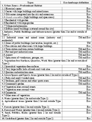
Types Eco-landscape definition 1. Urban Zones Predominant Habitat
1.1 Historical center Eco
1.2 Center with large buildings and mixed zones Eco
1.3 Old centers integrated into the city and extensions Eco
1.4 Grandsensembles (high buildings and open areas) Eco
1.5 Residential with garden Eco
1.6 Residential with large garden Eco
1.7 Village and extensions Eco
1.8 Diffuse (small buildings scattered around the city) Eco
2. Industry, Public Buildings and Infrastructures (greater than 2 ha and/or outside of Type 1)
2.1 Industrial zones and mixed zones (industry and residential)
TM and Eco
2.2 Zones of public buildings (universities, hospitals, etc.) TM
2.3 Fire stations and other areas with large buildings Eco
2.4 Train station and train station buildings TM and Eco
2.5 Port and port industrial zone TM and Eco
2.6 Airport TM and Eco
2.7 Open areas of warehouses, garages, etc. TM and Eco
3. Vegetation-free Surfaces, Quarries, Work Sites (greater than 2 ha and/or outside of Type 1)
3.1 Interstitial vegetation-free surfaces Eco
3.2 Very large traffic hubs of roads and work sites TM and Eco
3.3 Quarries and extraction areas TM and Eco
4. Green Spaces and Sports Areas (greater than 2 ha and/or outside of Type 1)
4.1 Parks and small wooded areas TM and Eco
4.2 Stadiums, golf courses and other sports areas TM and Eco
4.3 Community garden TM and Eco
4.4 Vegetation areas around streets Eco
4.5 Vegetation areas around water Eco
4.6 Cemeteries TM and Eco
4.7 Other areas of vegetation Eco
5. Water (greater than 2 ha and outside Type 1) Eco 6. Agricultural Areas (greater than 2 ha and outside Type
10. Undefined (greater than 2 ha and outside Type 1) Eco
6.2.5. Building the landscape analysis grid
At the end of this eco-landscape analysis, and once the map is produced, the objective is to build an analysis grid that will allow the introduction of survey and observation data from individuals, who, in the end, are the ones who will allow us to identify the signifier of environmental values.
The methodological requirements are based on the fact that:
the eco-landscape data correspond to highly heterogeneous zones with regard to form and size;
that the data from the representations are geo-referenced as points; and
that the behavioral data can be identified either ad hoc (address) or within a network defined by the researcher.
In other words, each type of data tends to ignore the format of the others. Therefore, the methodological objective involves harmonizing the spatial unit of these three types of data so as to be able to qualify the landscape context of visited and represented places based on the same procedure. Establishing relationships between these data is then possible by using the network found in the detailed city-plan booklet for the urban space being studied (a commercial booklet for addresses in order to meet daily needs).
Choosing this grid provides many advantages. On one hand, it is easy to use at the time when the respondent codes the site he/she visited, which allows him/her to maintain a certain level of confidentiality regarding his/her private life and to easily code the same place. Indeed, the coding procedure is identical to the procedure for searching for an address in daily life. On the other hand, grid regularity offsets the irregularities in form and size of the landscape map. Lastly, the cells allow us to qualify the context of the places visited or represented on the basis of an expanse rather than on that of a punctual spatial correspondence between a represented or visited urban element and its landscape attributes. This choice is due to the fact that the concept of landscape implies qualifying a space on the basis of an area, since our focus is on the landscape context for the urban element recorded in the survey, and not only on the quality of the element insertion point. Therefore, the cell becomes the spatial unit for data analysis an analysis unit that must initially be qualified from a landscape point of view.
The spatial intersection of the grid used with the urban eco-landscape map allowed us to qualify each cell, knowing that each of them is very often composed of several types of landscapes. A classification based on the proportion of landscape surfaces recorded in each cell allowed us to show the main landscape qualities making them up. Six types of cells were identified using the following criteria:
– uniform cells: cells with 95100% of their surfaces covered by a single type of landscape;
– predominance cells: cells having landscapes that cover at least 50%, and at most 94.9%, of the surface, even if other landscapes are present;
– minor predominance cells: cells having one type of landscape covering 4050% of the cell surface, and whose proportion of other landscapes is at least 10 points less than the predominant landscape;
– concomitance cells: cells having two types of landscape each covering 50% of the cell surface, with a maximum difference of 10 points more or less than 50% for each type of landscape;
– minor concomitance cells: cells having two or more types of landscape with a difference of more than 10 points between them;
– other cells: these are generally cells with a landscape surface of <10% of the total area of the cell, or that do not correspond to any of the other cell categories.
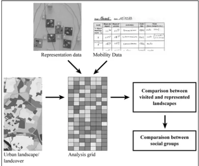
Figure 6.1. General procedure for landscape analysis
Qualification of the overall grid on the basis of the landscape map is the tool that allows us to compare represented landscapes and visited landscapes, as well as social groups.
6.3. Behavioral and representational data collection
The survey method makes use of a semi-structured interview, a questionnaire and respondent self-observation. It requires an initial face-to-face meeting lasting at least 90 minutes, and then three telephone interviews, each of approximately 15 minutes. Searching for complementary information on the signified of the environmental values is possible; this implies adding a second semi-structured face-to-face interview to identify reflexive data based on response time used.
The face-to-face meeting consists of a questionnaire for initially identifying the sociodemographic characteristics, residential mobility of the individuals and the level of equipment in the household. The person is then invited to express his/her representation of the space using a simple model that records the spatial organization of environmental knowledge. The final stage in the interview involves training the respondent in the self-observation of his/her mobility behavior over seven consecutive days following the meeting. The telephone interviews take place during this self-observation phase.
6.3.1. The spatial reconstruction set (JRS5): a cognitive spatial representation data
collection technique
The objective of this task involves recording the urban elements that make up the individual’s spatial representation. Freehand drawing is the most common technique. It has been used for more than 40 years in various fields, such as geography, sociology, anthropology and psychology. It has the enormous advantage of being inexpensive in terms of the materials required (paper and pencil). Moreover, the procedures for carrying it out are simple and easily adapted to different survey situations (individually or in a group, on different sites, etc.). Lastly, the respondent can potentially refer to the scale of his/her choice in his/her response. It has many methodological biases, however, since drawing is a highly discriminating form of expression from the point of view of social groups [RAM 06a]. It implies having either previously integrated the graphic codes of mapping or developed a graphic language in situ that is accepted by both the investigator and the respondent. This situation limits the expression of spatial knowledge and tends to lead to a self-censuring of knowledge in certain groups.
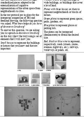
The JRS consists of a series of eight standardized pieces adapted to the externalization of cognitive
representations of the urban space from neighborhoods to cities.
In the test protocol put in place for the intergroup comparison of JRS and freehand drawing, the following question was asked: What knowledge do you have of downtown Strasburg?
To answer this question, we are asking you to reproduce downtown Strasburg on this tray (show the tray) using a set of elements that I will show you:
Small houses to represent the buildings or houses that you know and that are important.
Wooden blocks to represent high or wide buildings, or buildings that cover a lot of land.
Plates with three houses on them to represent neighborhoods or blocks of houses.
Green plates to represent green spaces, parks, gardens, etc.
Blue plates to represent places or parking lots.
The plates can be juxtaposed (demonstrate) to obtain the desired size.
Red, black or blue wire to represent, respectively, roads (streets, routes, avenues, highways, etc.), railways, waterways or ponds, etc.
Furthermore, the fact that this type of expression uses “paper and pencil” strongly differentiates respondents, since the relationship to this type of task is highly dependent upon the individual’s level of education. This is significant to the point that certain groups are more reluctant than others to carry out this exercise, which definitively amounts to putting them in the position of failing. The alternative involves using a modeling task, in this case the spatial reconstruction set (JRS), in order to improve expression of the cognitive representation of space and the comparisons between social groups [RAM 06a].
This game, made up of eight series of standardized pieces (see Figure 6.2), enables the individual to use a relatively flexible “language” to express the overall environmental knowledge making up his/her spatial representation. Consequently, the mental loading required for this exercise is lightened, which reduces the bias generally introduced in the paper-and-pencil task. Lastly, the limited number of pieces allows us to use the set with highly diverse populations in terms of age. Thus, this technique can be used from six years of age [RAM 06b] well into senior years [RAM 06c]. Moreover, the standardization of JRS pieces allows for comparisons that are often difficult to make using a drawing. It is therefore easier for the investigator to directly carry out quantitative analyses (number and types of elements represented, etc.) and qualitative analyses (comparison of spatial structures regardless of graphic style).
This technique, more appreciated than drawing [RAM 06a], also allows the respondent to adjust the position of the urban elements mentioned while moving the pieces. Each time that an element is put on the tray, it is numbered using a pre-printed label, and the investigator notes its identifier as formulated by the respondent.
The instructions are very open-ended and focused on the spatial knowledge of individuals. Their execution is limited to 15 minutes, since only the main urban elements are useful to the analysis. The spatial production is then photographed and archived.
6.3.2. Collecting travel behavior data
declared responses emphasize the behaviors that reflect common sense and social representations, or that are strongly filtered by the social desirability effect, unbeknownst to the two people involved in the survey. Lastly, the disassociation between verbal behavior and spatial behavior accentuates both the omissions and selections taken from memory [AUR 96]. Therefore, doubting the truthfulness of the response is not what is important; rather it is getting beyond biases from the investigator and respondent that stem from the social situation that the survey inevitably implies.
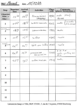
Direct behavior observation is also too expensive, if not impossible, to carry out without technological input (e.g. GPS) when the observation place is not stable and unique. We believe that the trip log technique is the most appropriate solution for identifying spatial behaviors, especially because we had chosen to identify all mobility behavior over a full week. This tool is based on an indirect observation method in which the respondent observes him/herself. It is only when he/she recounts his/her self-observations that the survey situation comes into play with its methodological biases.
The benefit of this tool is that it does not separate verbal behavior from spatial behavior. Therefore, it is easier for the person taking the survey to refuse this type of method or to stop the procedure, often on the pretext that the process is too cumbersome, than to consciously or unconsciously get involved in a social game. For the investigator, it is thus easier to see the difficulties that individuals encounter in recounting their behaviors. The fact that the respondent observes him/herself without the control of the investigator is another considerable benefit. Yet another asset is the length of the behavior observation period. While an interview only allows us to look at the behaviors of the day before the meeting, self-observation allows us to easily piece together those of an entire week. The final advantage of this method is the possibility of collecting trips whose reasons are insignificant for the respondent (mailing a letter, talking to a neighbor in the street, etc.) and that are difficult to detect with GPS (stop time often too short). This implies a simple instruction for the respondent (e.g. note all your trips outside the home).
The main disadvantage of this method is the tediousness of the procedure, especially when the self-observation period exceeds two consecutive days. It generally results in simplifying the filling in of the log, repeating the routine activities periods in both time and space (e.g. work) and, gradually, leaving out small “insignificant” trips.
of these seven pages is dated when it is presented. The respondent is instructed to use this log as a reference. He/she is encouraged to keep it with him/her during travel. The document can be folded, erased and scribbled on. The respondent must note the hours that he/she leaves and arrives at an activity outside his/her home. The activity is defined by a stop, even if it is brief or impromptu (stopping to talk to a friend on the sidewalk, for example).
The respondent is then asked to code, every evening, all of places where each activity took place using the booklet with detailed maps of the city being studied, which is offered to him/her at the end of the observation period. Coding involves noting the page number and then the reference in the cell in which the activity took place; this reference generally comprises a letter and number (e.g.: 19A1 for page 19 and cell A1). This coding is taught when the log is handed out. Every 48 hours, the investigator reaches the respondent at the time of the telephone meeting set up previously, to find out for each activity the times, place-code, transportation mode, people who were with the person taking the survey during the travel and activity. The telephone interview enables us to prevent the respondent from growing tired of using the tool and also to check for any possible “holes” along the way in time-use taken and declared.
6.4. Behavioral and representational data processing
We must keep in mind that the purpose of the analysis is to understand the eco-landscape characteristics of places visited and represented in order to find the signifier of the environmental values involved in people’s daily mobility.
6.4.1. The processing of visited places
From the time of the interview, insofar as the spatial reference is the cell, it is possible to directly geo-reference the places visited the on the basis of the geographical unit of analysis described above. This spatial coding allows us to collect two types of information:
– information on the spatial structure of the places visited, which corresponds to their spatial distribution (focused around the home, spread over a sector of the urban area, etc.);
– information on landscape qualities associated with the places visited.
These qualities allow us to obtain a landscape profile for each group:
– on all places visited during the week without taking frequency into account;
– on all places visited by weighing the landscape quality by visit frequency;
– or on places visited for each type of activity.
Activity coding can be broken down into seven categories:
– service activities (use of public or private services: hairdresser, mechanic, dyer, photo agency, etc.);
– visits (any activity to a private address in one’s social network);
– association activities (clubs, courses);
– religious activities (denominations, cemetery);
– recreational activities (sports, artistic activity, restaurants, cafés); and
– support activities (going with or picking up a member from the social network).
6.4.2. The processing of space cognitive representations
The first processing step involves distinguishing the points (specific places on the reduced scale and with identifiable contours, such as a park, a building), lines (thoroughfares) and neighborhoods in order to analyze the landscape quality for points alone. This choice is essentially guided by the current possibilities of using the lines and polygons with this type of landscape analysis grid. Indeed, thoroughfares, just like neighborhoods, are not urban elements whose cognitive reality corresponds to an administrative reality. Therefore, their limits cannot be specifically located6. Moreover, a large number of thoroughfares generally cannot
be identified at all, because they are either unnamed or are based on their daily function (the street to go to the supermarket). However, we are seeking to develop methods that will offset these problems.
The first product of this processing is a pattern of dots (in the form of a GIS layer), which intersected with the landscape analysis grid allows us to associate a cell in the grid with each of them. The format of this set of dots is the same as that for data from places visited. On one hand, the landscape analysis is carried out using the same protocol, i.e. using the quality of the cell as the analysis unit, and on the other hand the places represented and places visited can be compared.
Complementary processing of cognitive representations is possible. Indeed, we can qualify the spatial structure of the representation by using the general form of the representation based on:
6 For thoroughfares, particularly when they are long, only a portion of the road or boulevard has a psychological reality for the individual. For neighborhoods, should we base ourselves on administrative limits (which generally have no meaning for the respondent) or morphological limits, at the risk of over-interpreting the elements present in the cognitive representation, etc.?
– the order that elements appear (did the respondent start his representation with the neighborhoods, thoroughfares or specific elements?);
– the type of identification of elements (common name, functional identification); and
– the proportion of thoroughfares, neighborhoods and specific elements.
This processing does not provide any direct information on environmental values. In particular, it allows us to complete the analysis of individuals’ relationships with the urban space as a whole by looking further at the relationship between representation and spatial behaviors.
6.5. An application example: the Cronenbourg district pensioners’ mobility
An exploratory analysis of the relationship between daily mobility and urban eco-landscapes was carried out with 19 retirees, over 60 years of age, all living in a residential suburb near Strasburg: the Saint Antoine sector, built in the 1950s to 1960s in the Cronenbourg neighborhood.
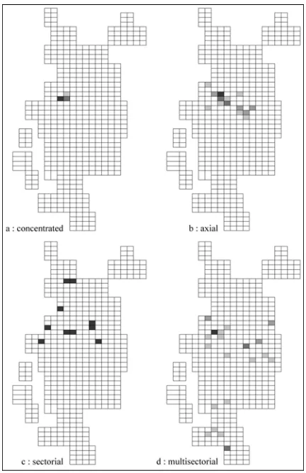
The eco-landscape throughout the urban community of Strasburg enabled us to produce the typology presented in Table 6.1. A total of 769 trips were identified. The spatial structure of mobility led to distinguishing four groups of individuals, as illustrated in Figure 6.4:
– those who visited places that are primarily concentrated around the home (concentrated distribution);
– those who visited places that form an axis between the home and downtown (axial distribution);
– those who visited places that are limited to a sector of the city and suburbs (sectorial distribution);
– those who visited places that are spread over several sectors of the city and suburbs (multisectorial distribution).
with large buildings, large-scale public buildings (hospital, university, etc.) and parks.
Figure 6.4. Examples of the spatial structure of mobility four remarkable distributions
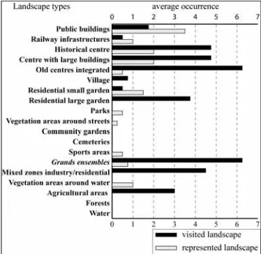
When distribution is axial, the landscapes represented seem to conflict with the landscapes visited (see Figure 6.5). Indeed, when the heritage landscapes (historical center, downtown made up of large buildings, old centers integrated into the current urban fabric) are highly visited, it is the sectors where public buildings predominate that are represented. Moreover, seven types of landscapes are either only represented or only visited. Two types of environmental values seem to appear. First, heritage environmental values based on both the representation and visiting of places. Second, functional environmental values in the suburbs from both the landscape point of view (grands ensembles, mixed residential-industrial zone) and the property point of view (essentially behavioral base).
Unlike the first group, when trip distribution is multisectorial, the urban heritage landscapes become more apparent in the representation than they are actually visited (see Figure 6.6). Isolated villages are visited without, however, being mentioned in the representation of the city. Also, urban forests, and especially landscapes made up of houses with large gardens, community gardens, grands ensembles and sports centers in the surrounding areas do not appear in the representation, even though they are visited. Here the environmental values are in opposition with the heritage city in terms of nature and greenery, the first being identitary, with the second having a strong behavioral basis.
Figure 6.6. Comparison of average occurrences between landscapes represented and landscapes visited for multisectorial distributions
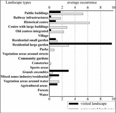
When the distribution of weekly trips is concentrated (see Figure 6.7), as for the previous group, the representation is essentially made up of ad-hoc elements from all urban heritage landscapes, while the landscapes visited are strongly limited to residential areas with large gardens. Here, the environmental values are essentially based on urban vegetation and residential areas, along with a strong urban identity.
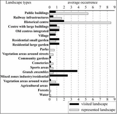
Lastly, when the spatial distribution of trips is sectorial (see Figure 6.8), the landscapes visited are concentrated in the grands ensembles and the mixed industrial-residential zones, whereas the landscapes represented are primarily urban historical landscapes found downtown. Here the environmental values are essentially urban, with a symbolic heritage component on one hand and a functional suburb component on the other.
Figure 6.8. Comparison of average occurrences between landscapes represented and landscapes visited for sectorial distributions
This example, which comes out of an exploratory study on a few individuals that are specific because of their age, shows major differences in the morphology of the places visited, although the entire sample lives in the same neighborhood and in the same type of housing. In order for the environmental values that confirm these differences to be more explicit, more advanced statistical analyses (comparisons of averages, multivariate analysis of variance, AFCM, ACP, etc.) should be carried out in order to better understand the structure of data collected, which this sample did not allow us to do. Adding an interview at the end of the self-observation phase
would also help identify certain dimensions of the signified for environmental values, in particular using the spatiotemporal grid for the level of spontaneity of trips [RAM 05].
This example shows that the signifiers for the environmental values can be described by simultaneously taking into account their cognitive or behavioral dimensions.
The sociological dimension should not be ignored. Indeed, the level of education of the respondents is the variable that appears to best explain the four empirically formed groups of citizens. An analysis of a larger sample would allow us to statistically ascertain this and would open up other avenues of exploration regarding the link between daily trips and sociospatial segregation. Moreover, a larger sample would allow us to carry out more in-depth analyses by studying each trip mode separately, by comparing them or even comparing the results obtained based on the classes of activities behind the trip.
6.6. Conclusion
Understanding urban forms that are associated with daily trips is a problem to which several studies have attempted to find answers. Indeed, the questions associated with this scientific challenge are at the heart of those on urban planning. They primarily concern issues of equal access by city-dwellers to urban resources (businesses, public and private services, urban amenities, etc.) from their home, to itineraries taken during trips, but also to the pollution that intra-urban daily trips entail. All these urban development issues pose the problem of the relationship between urban morphology and spatial behaviors. However, environmental values internalized by the individual are crucial for analyzing this relationship.
The investigation of environmental values associated with daily trips definitely allows us to search for solutions to the main problems produced by dominant urban practices. These studies are thus based on a definition of the urban space that is formulated around movement: “urbanization is defined here as the process in which mobility organizes daily life” [REM 92]; “urban is movement” [BAS 01]. Lastly, the convergence of psychological, geographical and sociological aspects implies that we no longer separate the effects of places, social groups and representation in the analysis of intra-urban daily movement.
6.7. Acknowledgements
The methodological developments presented in this chapter are from the research project Morphologies de l’étalement urbain et exclusion par l’automobilité (morphology of urban sprawl and exclusion by automobility, scientific coordinator: D. Pinson) for the Sustainable Urban Development Program at the CNRS. They are also taken from the research project Approche éco-paysagique révélatrice des identités de déplacement: une contribution interdisciplinaire à l’éco-développement urbain (eco-landscape approach reveals movement identities: an interdisciplinary contribution to urban eco-development, scientific coordinators: T. Ramadier and L. Wassenhoven) of EGIDE’s Platon Program. The two projects were conducted at the Laboratoire Image et Ville (UMR 7011 CNRS/ULP), at Louis-Pasteur University in Strasburg.
6.8. Bibliography
[APP 69] APPLEYARD D., “Why buildings are known”, Environment and Behavior, vol. 1, pp. 131-159, 1969
[AUR 96] AURIAT, N., Les Défaillances de la Mémoire Humaine: Aspects Cognitifs des Enquêtes Rétrospectives, Paris, PUF, 1996
[BAI 90] BAILLY A., “Paysages et representations”, Mappemonde, vol. 3, pp. 10-13, 1990
[BAS 01]BASSAND M., “Métropole et métropolisation”, in: BASSAND M.,KAUFMANN V., JOYE D. (eds), Enjeux de la Sociologie Urbaine, Lausanne, Romandes Polytechnic and University Press, 2001
[BER 95] BERQUE A., Les Raisons du Paysage de la Chine Antique aux Environnements de Synthèse, Vanves, Editions Hazan, 1995
[BOU 79] Bourdieu P., La Distinction, Paris, Editions de Minuit, 1979
[BRO 84] BROSSARD T., WIEBER J.C., “Le paysage: trois définitions, un modèle d’analyse et de cartographie”, L’Espace Géographique, vol. 1, pp. 5-12, 1984
[CLA 95] CLAVAL P., La Géographie Culturelle, Paris, Nathan, 1995
[FIN 68] FINES K.D., “Landscape evaluation: A research project in East Sussex”, Regional Studies, vol. 2, pp.41-55, 1968
[HAR 72] HARRISON J.D., HOWARD W.A., “The role of meaning in the urban image”, Environment and Behavior, vol. 4, pp. 389-411, 1972
[HER 03] HERZOG T. R, LEVERICH O.L., “Searching for legibility”, Environment and Behavior, vol. 4, pp. 459-477, 2003
[HER 76] HERZOG T. R., KAPLAN S., KAPLAN R., “The prediction of preference for familiar places”, Environment and Behavior, vol. 4, pp. 627-645, 1976
[HOI 71] HOINVILLE G., “Evaluating community preferences”, Environment and Planning, vol. 3, pp. 33-50, 1971
[KAP 87] KAPLAN S., “Aesthetics, affect and cognition: Environmental preferences from an evolutionary perspective”, Environment and Behavior, vol. 1, pp. 3-32, 1987
[KES 01] KESTENS Y., THÉRIAULT M., DES ROSIERS F. “Nature de l’utilisation du sol et valeurs immobilières résidentielles : analyse par modélisation hédonique”, Les Cahiers du GRATICE, vol. 21, pp. 111-141, 2001
[LYN 60] LYNCH K., The Image of the City, Cambridge, Mass., MIT Press, 1960
[MAT 88] MATALON B., Décrire, Expliquer, Prévoir. Démarches Expérimentales et Terrain, Paris, Armand Colin, 1988
[PET 03] PETROPOULOU C., Étude comparée des changements périurbains. Les quartiers spontanés à Athènes et à Mexico, Human geography doctorat thesis, Louis Pasteur University, Strasbourg, 2003
[PET 06] PETROPOULOU C., PANGAS N., “ȋȦȡȠIJĮȟȚțȒʌȡȠıȑȖȖȚıȘIJȠȣʌİȡȚĮıIJȚțȠȪȤȫȡȠȣȝİ ȕȐıȘIJȘȞIJȠʌȚȠ-ȠȚțȠıȣıIJȘȝȚțȒșİȫȡȘıȘ (Urban planning approach of peri-urban space based in landscape ecology theory)”, īİȦȖȡĮijȓİȢ (Geographies), vol. 12, 2006
[RAM 98] RAMADIER T., MOSER G., “Social legibility, the cognitive map and urban behavior”, Journal of Environmental Psychology. vol. 3, pp. 307-319, 1998
[RAM 05] RAMADIER T., LEE-GOSSELIN M., FRENETTE A., “Conceptual perspective for explaining spatio-temporal behaviour in urban areas”, in LEE-GOSSELIN M.E.H., DOHERTY S.T (Eds) Integrated land-use and Transportation Models: Behavioural Foundations, Elsevier, Oxford, pp. 87-100, 2005
[RAM 06a] RAMADIER T.; BRONNER A.C., “Knowledge of the environment and spatial cognition: Jrs as a technique for improving comparisons between social groups”, Environment and Planning B: Planning and Design, vol. 33, pp. 285-299, 2006
[RAM 06b] RAMADIER T., DEPEAU S., “Approche méthodologique (JRS) et développementale de la représentation de l’espace quotidien de l’enfant”, presented at International Pluridisciplinaire Les Enfants et les Jeunes dans les Espaces Quotidiens, Rennes, November 2006
[RAM 06c] RAMADIER T., PETROPOULOU C., HANIOTOU H., BRONNER A.C., ENAUX C., Morphologie de l’Étalement Urbain et Exclusion par l’Automobilité: le Cas des Adolescents et des Personnes âgées de Cronenbourg, une Banlieue de l’Agglomération de Strasbourg, CNRS, program of durable urban development, Strasbourg, June 2006
[RAS 69] RASER , J.R., Simulation and Society: an Exploration of Scientific Gaming, Boston, Allyn & Bacon, 1969