Zhirong Yang2 [email protected]
Jaakko Peltonen1,4 [email protected]
Samuel Kaski1,3 [email protected]
1Helsinki Institute for Information Technology HIIT,2Department of Information and Computer Science, Aalto University,
Finland,3Department of Computer Science, University of Helsinki, and4University of Tampere
Abstract
Visualization methods that arrange data objects in 2D or 3D layouts have followed two main schools, methods oriented for graph layout and methods oriented for vectorial embedding. We show the two previously separate approaches are tied by an optimization equivalence, mak-ing it possible to relate methods from the two approaches and to build new methods that take the best of both worlds. In detail, we prove a theorem of optimization equivalences between β- andγ-, as well asα- and R´enyi-divergences through a connection scalar. Through the equiv-alences we represent several nonlinear dimen-sionality reduction and graph drawing methods in a generalized stochastic neighbor embedding setting, where information divergences are min-imized between similarities in input and output spaces, and the optimal connection scalar pro-vides a natural choice for the tradeoff between attractive and repulsive forces. We give two ex-amples of developing new visualization meth-ods through the equivalences: 1) We develop weighted symmetric stochastic neighbor embed-ding (ws-SNE) from Elastic Embedembed-ding and ana-lyze its benefits, good performance for both vec-torial and network data; in experiments ws-SNE has good performance across data sets of dif-ferent types, whereas comparison methods fail for some of the data sets; 2) we develop a γ -divergence version of a PolyLog layout method; the new method is scale invariant in the output space and makes it possible to efficiently use large-scale smoothed neighborhoods.
Proceedings of the 31st
International Conference on Machine Learning, Beijing, China, 2014. JMLR: W&CP volume 32. Copy-right 2014 by the author(s).
1. Introduction
We address two research problems: nonlinear dimension-ality reduction (NLDR) of vectorial data and graph layout. In NLDR, given a set of data points represented with high-dimensional feature vectors or a distance matrix between such vectors, low-dimensional coordinates are sought for each data point. In graph layout, given a set of nodes (ver-tices) and a set of edges between node pairs, the task is to place the nodes on a 2D or 3D display. Solutions to both research problems are widely used in data visualization.
The two genres have yielded corresponding schools of methods. To visualize vectorial data, many NLDR meth-ods have been introduced, from linear methmeth-ods based on eigendecomposition, such as Principal Component Anal-ysis, to nonlinear methods such as Isomap or Locally Linear Embedding. Recent well-performing methods in-clude Stochastic Neighbor Embedding (SNE; Hinton & Roweis,2002), Neighbor Retrieval Visualizer (Venna et al.,
2010), Elastic Embedding (EE; Carreira-Perpi˜n´an,2010), Semidefinite Embedding (Weinberger & Saul,2006), and the Gaussian process latent variable model (Lawrence,
2003). However, these methods often yield poor embed-dings given network data as input, especially when the graph nodes have heavily imbalanced degrees.
Force-based methods are probably the most used graph lay-out method family. They set attractive forces between ad-jacent graph nodes and repulsive forces between all nodes, and seek an equilibrium of the force system analogous to having springs attached between nodes. The methods typ-ically modify an initial vertex placement by iteratively ad-justing vertices. Many layout methods have been proposed, such as sfdp (Hu,2005), LinLog (Noack,2007), OpenOrd (Martin et al.,2011), and MaxEnt (Gansner et al.,2013). The methods can be used for vector-valued data as well, transformed into a neighborhood graph, but have not been designed for that task and often do not find good low-dim-ensional embeddings for high-dimlow-dim-ensional neighborhoods.
ex-pressed as optimizing a divergence between neighborhoods in the input and output spaces, collectively called Neighbor Embedding (NE;Yang et al.,2013). Two common kinds of NE objectives are 1) using a separable divergence1 on
non-normalized neighborhoods, as in e.g. EE, and 2) using a nonseparable divergence on normalized neighborhoods, as in e.g. SNE. However, it remains unknown whether the two kinds of objectives are essentially equivalent.
In this paper we address the question by introducing novel relationships between the objectives. We prove an opti-mization equivalencebetween a separable divergence (αor β) and its corresponding nonseparable divergence (R´enyi orγ) through an optimizable connection scalar. This theo-rem provides a connection between common NLDR and conventional force-directed methods, allowing develop-ment of more general and robust visualization methods by using extensions and insights from either side. Separable force-directed objectives are easier to design and optimize, but the tradeoff between attraction and repulsion as a hy-perparameter is hard to determine. On the other hand, ob-jectives formulated with R´enyi- orγ-divergence are scale invariant. Moreover, the optimal connection scalar yields a principled choice for the attraction-repulsion tradeoff.
We demonstrate two applications of the optimization equivalence. First, we introduce a weighted variant of sym-metric SNE (ws-SNE) by integrating the “edge-repulsion” strategy from the force-directed graph layout algorithms and applying the optimization equivalence which automat-ically selects the best tradeoff between attraction and repul-sion. Experiments show thatws-SNE works well for both vectorial and network data, whereas the other compared neighbor embedding or graph drawing methods achieve good results for only one of the two types of data. The su-perior performance of ws-SNE is explained through the op-timization equivalence. Second, we develop a new variant of the PolyLog method that minimizes the γ-divergence. This new method is invariant to scale of the mapped points and allows large-scale smoothed input neighborhoods.
We review popular divergence measure families in Section
2. We introduce the optimization equivalence theorem in Section3and the neighbor embedding framework in Sec-tion 4. We introduce the new visualization methods and their analysis in Section5, and show their goodness by ex-perimental comparisons in Section6. Section7concludes.
2. Divergence measures
Information divergences, denoted byD(p||q), were origi-nally defined for probabilities and later extended to
mea-1
A separable divergence here means a divergence that is a sum of pairwise terms, where each term depends only on locations of one pair of data.
sure difference between two (usually nonnegative) tensors pandq, whereD(p||q)≥0andD(p||q) = 0iffp=q. To avoid notational clutter we only give vectorial definitions; it is straightforward to extend the formulae to matrices and higher-order tensors. We focus on four important families of divergences: α-, β-, γ- and R´enyi (parameterized by r). Their definitions are (see e.g. Cichocki et al.,2011):
Dα(p||q) = 1
where pi and qi are the entries in p and q respectively, ˜
pi = pi/Pjpj, and q˜i = qi/Pjqj. To handle p’s containing zero entries, we only consider nonnegative α, β, γ and r. These families are rich as they cover most commonly used divergences in machine learning such as
DKL(p||q) =X note normalized Kullback-Leibler (KL) divergence, non-normalized KL-divergence and Itakura-Saito divergence, respectively. Other named special cases include Euclidean distance (β = 2), Hellinger distance (α = 0.5), and Chi-square divergence (α= 2). Different divergences have be-come widespread in different domains. For example,DKL is widely used for text documents (e.g. Hofmann,1999) and DIS is popular for audio signals (e.g. F´evotte et al.,
2009). In general, estimation usingα-divergence is more exclusive with largerα’s, and more inclusive with smaller α’s (e.g.Minka,2005). Forβ-divergence, the estimation becomes more robust but less efficient with largerβ’s.2
3. Connections between divergence measures
Here we present the main theoretical result. Previous work on divergence measures has mainly focused on re-lationships within one parametrized family. Little research has been done on the inter-family relationships; it is only known that there are correspondences betweenDαandDr, as well as betweenDβ andDγ (see e.g.Cichocki et al.,
2
2009). We make the more general connection precise by a new theorem ofoptimization equivalence:
Theorem 1. Forpi≥0,qi ≥0,i= 1, . . . , M, andτ≥0,
The proof is done by zeroing the derivative of the right hand side with respect toc(details in the appendix). The optimal cis given in closed form:
c∗= arg min
The optimization equivalence not only holds for the global minima but also all local minima. This is justified by the following proposition (proof at the end of the Appendix): Proposition 2. The stationary points ofDγ→τ(p||q)and minc≥0Dβ→τ(p||cq), as well as of Dr→τ(p||q) and
minc≥0Dα→τ(p||cq), in Theorem1are the same.
To understand the value of the above theorem, let us first look at pros and cons of the four divergence families. The γ- and R´enyi divergences are invariant of the scaling ofp andq, which is desirable in many applications. However, they are not separable over the entries which increases opti-mization difficulty, and it is more difficult to design variants of the divergences due to the complicated functional forms. On the other hand,α- andβ-divergences are separable and yield simpler derivatives, thus stochastic or distributed im-plementations become straightforward. However, the sep-arable divergences are sensitive to the scaling ofpandq.
Theorem 1 lets us take the advantages from either side. To design a divergence as a cost function for an applica-tion one can start from the separable side, inserting opti-mization and weighting strategies as needed, for example based on analyzing the resulting gradients, and then for-mulate the final scale-invariant objective by aγ- or R´enyi-divergence and analyze its properties (see an example in Section5.1). In optimization, one can turn back to the sep-arable side and use efficient algorithms. In visualization, we show below that the scalarc(denoted λin Section 4) controls the tradeoff between two learning sub-objectives corresponding to attractive and repulsive forces. Unlike in conventional force-directed approaches, here Theorem1
gives an optimization principle to adaptively and automati-cally choose the best tradeoff: in order to be equivalent to a scale-invariant objective, the objective is formulated as on the right-hand side of (1) or (2), and the optimal tradeoffc∗
is found as part of the minimization.
4. Neighbor Embedding optimizes
divergences
We present a framework for visualization based on in-formation divergences. We start from multivariate data and generalize to graph visualization in the next sec-tion. Suppose there are N high-dimensional data ob-jects {x1, . . . , xN}. Their neighborhoods are encoded in a square nonnegative matrixP, wherePij is proportional to the probability that xj is a neighbor of xi. Neigh-bor Embedding (NE) finds a low-dimensional mapping xi 7→ yi ∈ Rmsuch that the neighborhoods are approx-imately preserved in the mapped space. Usuallym= 2or 3. If the neighborhood in the mapped space is encoded in Q∈Rn×nwhereQijis proportional to the probability that yjis a neighbor ofyi, the NE task is to minimizeD(P||Q) overY = [y1, y2, . . . , yN]T for a certain divergenceD.
The formulation originated from Stochastic Neighbor Em-bedding (SNE; Hinton & Roweis, 2002). Let pij ≥
kqik. Typically qij is proportional to the
Gaus-sian distribution so that qij = exp −kyi−yjk2, or proportional to the Cauchy distribution so that qij = (1 +kyi−yjk2)−1 (i.e. the Studentt-distribution with a single degree of freedom).
Different choices of P, Q, and/or D give different NE methods. For example, minimizing a convex combination of Dr→1 andDr→0, that is, PiκDKL(Pi:||Qi:) + (1 − κ)DKL(Qi:||Pi:)withκ ∈ [0,1]a tradeoff parameter, re-sults in the method NeRV (Venna et al.,2010) which has an information retrieval interpretation of making a tradeoff between precision and recall; SNE is a special case (κ= 1) maximizing recall, whereasκ= 0maximizes precision. If the normalization is matrix-wise: Pij =pij/Pklpkl and Qij =qij/Pklqkl, minimizingDKL(P||Q)over Y gives a method called Symmetric SNE (s-SNE;van der Maaten & Hinton,2008). Whenqij = (1 +kyi−yjk2)−1, it is also called t-SNE (van der Maaten & Hinton,2008).
Although NE methods can be interpreted as force-directed methods, their design is different from conventional ones: in NE a divergence is picked, and forces between data arise from minimizing it. We distinguish SNE from conventional force-directed layouts because, by Theorem1, SNE pro-vides an information-theoretic way to automatically select the best tradeoff between attraction and repulsion.
Next we show that two other existing visualization methods can also be unified in the framework.
proposed EE which minimizes a Laplacian Eigenmap term (Belkin & Niyogi, 2002) plus a repulsive term:
JEE(Y) =Pijpijkyi−yjk2+λPijexp −kyi−yjk2, whereλcontrols the tradeoff between attraction and repul-sion3. The EE objective can be rewritten as J
EE(Y) = DI(p||λq) +C(λ), where qij = exp −kyi−yjk2
, and C(λ) = P
ijpij
lnλ−P
ij[pijlnpij−pij] is con-stant with respect to Y. Minimizing JEE over Y is thus equivalent to minimizing the separable divergence DI(p||λq) over Y. Notice that we do not optimize JEE overλ. This information divergence formulation also pro-vides an automatic way to chooseλby using Theorem1: arg minY[minλDI(p||λq)] = arg minY DKL(p||q), with the bestλ = P
ijpij/Pijqij. The non-separable diver-gence on the right-hand side is the s-SNE objective. Thus EE with the best tradeoff (yielding minimum I-divergence) is essentially s-SNE with Gaussian embedding kernels.
Proposition 4.Node-repulsive LinLog is a divergence min-imization method. Proof:Noack(2007) proposed the Lin-Log energy model which is widely used in graph draw-ing. The node repulsive version of LinLog minimizes
Jλ
LinLog(Y) =λ P
ijpijkyi−yjk −Pijlnkyi−yjk. Al-gebraic manipulation yields Jλ
LinLog(Y) = DIS(p||λq) + constant, whereqij =kyi−yjk−1.
A recent work (Bunte et al.,2012) also considers SNE for dimension reduction and visualization with various infor-mation divergences, but their formulation is restricted to stochastic matrices, and gives no optimization equivalence between normalized and non-normalized cases.
5. Developing new visualization methods
The framework and the optimization equivalence between divergences not only relate existing approaches, but also enable us to develop new visualization methods. We give two examples of such development: 1) a generalized SNE that works for both vectorial and network data, and 2) aγ -divergence formulation of PolyLog (Noack,2007) which is scale invariant in the output space and allows large-scale smoothed input neighborhoods. In both examples, Theo-rem1plays a crucial role in the development.
5.1. Example 1: ws-SNE
We want to build a method for a vectorial embedding but incorporating the useful edge repulsion (ER) strategy from graph drawing. ER would be easy to add to the EE ob-jective as it is pairwise separable. Borrowing the ER
strat-3
For notational clarity we only illustrate EE withw−
mn = 1
(seeCarreira-Perpi˜n´an,2010, Eq. 6). In his experiments Carreira-Perpi˜n´an(2010) also used uniformw−. It is straightforward to
extend the connection to the weighted version.
egy from Noack (2007), we insert weightsM in the re-pulsive term: Jweighted-EE(Y) = Pijpijkyi − yjk2 + λP
ijMijexp −kyi−yjk2
, where Mij = didj, and the vector dmeasures importance of the nodes. We use degree centrality as the measurement, i.e.,di=degree of the i-th node. Jweighted-EE(Y)has downsides: it needs a user-set edge repulsion weightλ, and is not invariant to scaling ofp. By Theorem1we create a corresponding improved method, ws-SNE, minimizing a nonseparable divergence.
Proposition 5. Weighted EE is a separable divergence minimizing method and its non-separable variant is ws-SNE. Proof: Writing qij = exp(−kyi − yjk2) with qii = 0, we have Jweighted-EE(Y) = DI(p||λM ◦ q) + F(λ), where ◦ denotes element-wise product and F(λ) = C(λ) + P
ijpijlndidj is a constant to Y. In the final and most important step, by a spe-cial case of Theorem 1: arg minY DKL(p||M ◦ q) = arg minY[minλ≥0DI(p||λM◦q)], we obtain a new vari-ant of SNE which minimizesDKL(p||M ◦q)overY:
Jws-SNE(Y) =− X
ij
pijlnqij+ ln X
ij
Mijqij+constant
We call the new method weighted symmetric Stochastic Neighbor Embedding (ws-SNE). As in SNE, other choices of qcan be used; for example, the Gaussianq can be re-placed by the Cauchyqij = (1 +kyi−yjk2)−1or other heavy-tailed functions (see e.g.Yang et al.,2009).
We used degree centrality as the importance measure for simplicity. Other centrality measures include closeness, be-tweenness, and eigenvector centralities. Note that for vec-torial data with K-Nearest-Neighbor (KNN) graphs, ws-SNE reduces to s-ws-SNE if out-degree centrality is used.
The ws-SNE method is related to the multiple maps t-SNE method (van der Maaten & Hinton,2011), but differently the latter aims at visualizing multiple views of a vectorial dataset by several sets of variable node weights. In addi-tion, ws-SNE does not impose the stochasticity constraint on the node weights. It is unknown whether multiple maps t-SNE can handle imbalanced degrees in graph drawing.
Analysis: best of both worlds. As shown by Proposi-tion 5, ws-SNE combines edge-repulsion merits from graph drawing with the scale-invariance and optimal attraction-repulsion tradeoff from SNE. We find it performs consis-tently well for vectorial and network data visualization.
are placed in the center (see Figure 1, C3 to C6 for ex-amples). In contrast, ws-SNE uses edge repulsion to handle such cases of imbalanced degrees. When the di are not uniform, ws-SNE behaves differently from con-ventional s-SNE, which can be explained by its gradient
∂Jws-SNE(Y) ∂yi =
P
jpijqijθ(yi−yj)−cdidjqij1+θ(yi−yj), wherec=P
ijpij/( P
ijdidjqij)is the connection scalar, andθ = 0 for Gaussianqandθ = 1 for Cauchyq. The first term in the summation is for attraction of nodes and the second for repulsion. Compared with the s-SNE gradi-ent, the repulsion part is weighted bydidjin ws-SNE. That is, important nodes have extra repulsive force with the oth-ers and thus tend to be placed farther. This edge-repulsion strategy has been shown to be effective in graph drawing to overcome the “crowding problem”, namely, many mapped points becoming crowded in the center of the display.
On the other hand, conventional graph drawing methods do not work well for multivariate data. They are usually de-signed by choosing various attractive and repulsive force terms, as in the “spring-electric” layout (Eades, 1984), Fruchterman-Rheingold (Fruchterman & Reingold,1991), LinLog (Noack, 2007), and ForceAtlas2 (Jacomy et al.,
2011). These force-directed models have a serious draw-back: the layout is sensitive to scaling of the input graph, thus the user must carefully (and often manually) select the tradeoff between attraction and repulsion. A constant trade-off or annealing scheme may yield mediocre visualizations.
The optimal tradeoff is automatically selected in ws-SNE by the optimization equivalence, yielding an objective in-variant to the scale ofp. This is more convenient and often performs better than conventional force-based methods.
Information retrieval interpretation. Venna & Kaski
(2007) andVenna et al.(2010) gave information retrieval perspectives of the unweighted SNE. As a new contribu-tion, we show in the supplement that ws-SNE optimizes vi-sualizations for a two-stage retrieval task: retrieving initial points and then their neighbors. In brief, we prove the cost can be written as a sum of divergences asJws-SNE(Y) = DKL({p˜i}||{q˜i}) +Pip˜iDKL({p˜j|i}||{q˜j|i})wherep˜i = P
kpik/Plmplmandq˜i = (diPkdkqik)/(Pkldkdlqkl) are marginal probabilities in the input and output space, and ˜
pj|i =pij/Pkpikandq˜j|i =djqij/(Pkdkqik)are con-ditional probabilities in the input and output space around pointi. The divergence between marginal probabilities is interpreted as performance of retrieving initial points; di-vergences between conditional probabilities are interpreted as performance of retrieving neighbors. In both stages the retrieval performance is mainly measured by recall (cost of missing points and their neighbors), and the weighting causes optimization to distribute high- and low-importance nodes more evenly.
5.2. Example 2:γ-QuadLog
In graph layout, smoothing graph adjacencies by random walks is potentially beneficial but computationally unfea-sible for many methods as smoothed adjacencies can be non-sparse. We use Theorem1to develop a layout method that efficiently incorporates random-walk smoothing.
A sparse input graph A can be smoothed by computing a random-walk transition probability matrix p = (1 −
ρ) I−ρD−1/2AD−1/2−1
with ρ ∈ (0,1) andDii = P
jAij. Smoothing can help layout methods avoid poor local optima and reveal macro structure of data. However, the matrixpis dense and infeasible to use explicitly in com-puting layout cost functions for large graphs. We start from QuadLog, a force-based method in ther-PolyLog family (Noack, 2007): Jλ
QuadLog(Y) = λ P
ijpijkyi −yjk2 − P
ijlnkyi−yjk2. While random walk smoothing can be applied in QuadLog, it is not scale-invariant and needs a user-set tradeoff parameterλ; we now solve this.
Proposition 6. QuadLog minimizes a separable diver-gence, and there exists an equivalent minimization of a non-separable divergence that still permits fast use of ran-dom walk smoothing. Proof: We show the QuadLog ob-jective is an Itakura-Saito divergence plus constants with respect to Y: simple manipulation gives Jλ
QuadLog(Y) = DIS(p||λq) +P
ijln(pij/λ) +N(N −1), where qij =
kyi−yjk−2. By Theorem1, minimizingJQuadLogλ (Y)with respect toλis equivalent to minimizingDγ→0(p||q). We
call the new methodγ-QuadLog as it is a counter-part of QuadLog in the γ-divergence family. Dropping the addi-tive constants, theγ-QuadLog objective is
Jγ-QuadLog(Y) = ln X
ij
pijkyi−yjk2− P
ijlnkyi−yjk2 N(N−1) . The new objective has two advantages: 1) It is scale-invari-ant in input and output: multiplyingpby a scaling factor does not change the optima; multiplyingY by a scaling fac-tor does not even change the objective value. 2) It allows use of smoothed neighborhood graphs: theγ-QuadLog ob-jective can be computed using the matrix productpY, and as in QuadLog,pY can be scalably computed by iterative approaches (e.g.Zhou et al.,2003, if random walk is used).
γ-QuadLog is the only method we know with both advan-tages 1) and 2). We could e.g. develop a scale-invariant ver-sion of node-repulsive LinLog (take the divergence form of
Jλ
LinLog(Y)from Proposition 4: by Theorem1, optimizing it w.r.t.λis equivalent tominY Dγ→0(p||q)) but it would
not allow efficient use of smoothed graphs.
6. Experiments
Log. For EE, ws-SNE, graphviz and LinLog, we used sym-metrized 10-NN graphs as input. For ws-SNE, we adopted the Cauchy kernel, spectral direction optimization ( Vla-dymyrov & Carreira-Perpi˜n´an,2012) and scalable imple-mentation with Barnes-Hut trees (van der Maaten,2013;
Yang et al.,2013). Both ws-SNE and t-SNE were run for the maximum 1000 iterations. We used default settings for the other compared methods (graphviz uses sfdp layout;
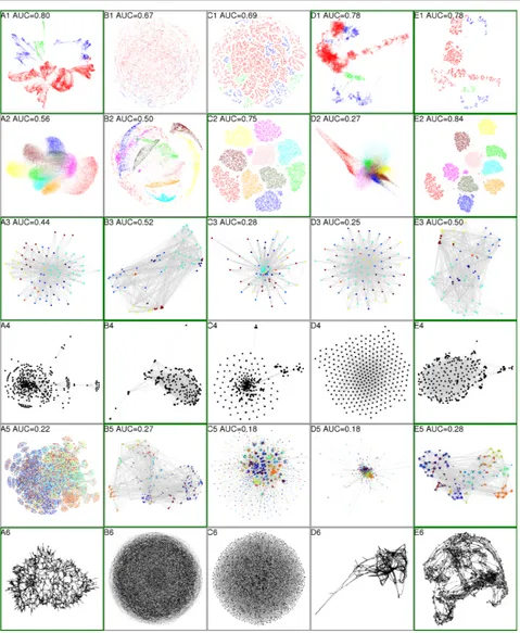
Hu,2005). The compared methods were used to visualize six data sets, two vectorial data and four network data. The descriptions of the data sets are given in the supplemental document. Figure1shows the resulting visualizations.
First let us look at the results for vectorial data. In a de-sired layout ofshuttleandMNIST, data points should be grouped according to ground truth classes shown as col-ors. In this respect, graphviz and ws-SNE are successful forshuttle. In contrast, LinLog fails badly by mixing up the classes in a hairball. In the t-SNE layout, the classes were broken up into unconnected small groups, without a meaningful macro structure being visible. ForMNIST, t-SNE and ws-t-SNE correctly identify most classes through clear gaps between the class point clouds; ws-SNE has even better AUC. In contrast, graphviz and LinLog perform much worse, heavily mixing and overlapping the classes.
Next we look at the visualizations of network data. For theworldtradedata set, a country generally has higher trading amounts with its neighboring countries. Therefore, a desired 2D visualization of the countries should correlate with their geographical layout. Here we illustrate the conti-nents of the countries by colors. We can see that graphviz, LinLog and ws-SNE can basically group the countries by their continents. In the high-resolution images annotated with country labels (in the supplemental document), we can also identify some known regional groups such as Scan-dinavian and Latin-American countries in the LinLog and ws-SNE visualizations. In contrast, Figure1 C3 shows a typical failure of t-SNE for graphs with imbalanced de-grees: the high-degree nodes are crowded in the middle while those with low degrees are scattered in the periphery.
In theusair97data set, the network links denote whether two cities have direct flights or not. A desired visualization of the data should correlate with geographical locations of the airports. LinLog and ws-SNE are more successful in this sense. We present the names of the 50 biggest airports (by degrees) in the supplemental document, where we see that the geographical topology is almost recovered in these two visualizations except southeast airports. In contrast, graphviz and t-SNE are problematic in this task, especially for placing continental airports; they tend to squeeze big airports in the middle and dangle small ones in periphery.
Formirex07, a desired visualization should be able to il-lustrate the music genres (shown as colors) of the songs.
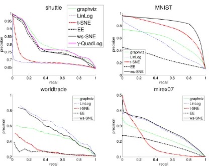
Figure 2.Recall-precision curves of the retrieval by KNN in the 2D space (with different K’s) for the four data sets with ground truth classes. Corresponding areas under the curve (AUCs) are shown in Figure1. This figure is best viewed in color.
LinLog and ws-SNE perform better for this purpose. In contrast, graphviz has a “broccoli-like” display which can only barely show the classes. The t-SNE method again suf-fers from the imbalanced degree problem: a lot of low-degree nodes occupy a large area and squeeze the high-degree nodes into the middle.
Forluxembourgthe ground truth is the geographical co-ordinates of the nodes as the edges are streets (see the sup-plemental document). However, visualization methods can easily fall into trivial local optima, for example, LinLog and t-SNE simply give meaningless displays like hairballs. In contrast, graphviz and ws-SNE successfully present a structure with much fewer crossing edges and higher re-semblance to the ground truth, even though the geographi-cal information was not used in their learning.
We fixedλ= 1in EE and the results are given in D1-D6 in Figure1. In this setting, EE only works well forshuttle and fails badly for all the other datasets. This indicates that EE performance heavily relies onλ. The EE layouts tend to be uniform with too largeλ’s (e.g. D3 and D4) or fail to unfold the structure with too smallλ’s (e.g. D2 and D6).
Besides qualitative results, we also quantify the visualiza-tion performance of data sets with ground truth classes. We plot the curves of mean precision vs. mean recall of retrieval in the KNN neighborhoods (in the visualization) across different K’s in Figure2. The area under the curves (AUCs) are shown in Figure1. The quantified results show that the ws-SNE method performs the best or very close to the best for the four data sets.
In summary, ws-SNE is the only method that gives good vi-sualizations over all the six data sets. The other four meth-ods can only discover the data structures in either some vec-torial or network data, but not over all data of both types.
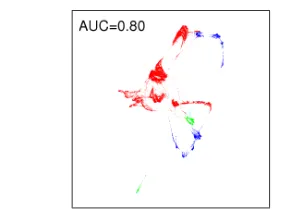
Figure 3.Visualization ofshuttleusingγ-QuadLog.
the shuttle dataset, where we used the random walk smoothing (ρ = 0.99) and gradient descent optimization, with the step size selected by backtracking to guarantee the cost function decreases. The visualization is given in Figure 3, and the ROC curve in Figure2 (top left). γ -QuadLog ties with graphviz as the best in retrieval perfor-mance (AUC). Note that zooming the display to a dense area as in EE and ws-SNE was not needed forγ-QuadLog.
7. Conclusions
We proved an optimization equivalence theorem between families of information divergence measures. The theorem, together with the known relationships within the families, provides a powerful framework for designing approxima-tive learning algorithms. Many nonlinear dimensionality reduction and graph drawing methods can be shown to be neighbor embedding methods with one of the divergences. As examples, we used the theorem to develop two new visualization methods. Remarkably, the ws-SNE variant works well for both vectorial and network data.
In this paper the divergence measure was selected man-ually. Methods exist to automatically select the best β -divergence (e.g.Simsekli et al.,2013;Lu et al.,2012). Our finding on divergence connections could extend the meth-ods toγ-divergence and toα- and R´enyi-divergences by a suitable transformation fromβtoα.
Both kinds of divergences have good properties: separa-ble divergences are easy to modify, thus we started method derivations from them, whereas non-separable divergences have appealing invariances and need no connection scalars. The benefit of changing to non-separable divergences is greatest when many connection scalars are needed on the separable side; in our examples the change got rid of a sin-gle tradeoff parameter, in cases involving many such pa-rameters the benefit would be even greater.
We gave preliminary empirical results of the two newly de-veloped methods. In ws-SNE, one could additionally use our framework and equivalence theorem to analyze effects of other centrality measures for the edge repulsion and even other weighting schemes. Theγ-QuadLog method will be tested on more datasets and with more advanced optimiza-tion methods in the future.
Acknowledgment
Academy of Finland, grants 251170, 140398, 252845, and 255725. Tekes Reknow project.
Appendix: proofs
Lemma 7arg minzaf(z) = arg minzalnf(z)fora∈R andf(z)>0.Proof: by the monotonicity ofln().
Proof of Theorem1. Next we prove the first part in The-orem 1. For τ /∈ {0,1}, ∂Dβ→τ(p||cq)/∂c = 0 gives alent to minimizing τ1ln(P
jqτj)− τ−11ln(
We can apply a similar technique to the second part in Theorem 1. ∂Dα→τ(p||cq)/∂c = 0 gives c∗ =
The proofs for the special cases are similar:
1)β = γ → 1(orα =r → 1): ∂Dβ→1(p||cq)/∂c= 0
gives c∗ = (P ipi)/(
P
iqi). Putting it back, we obtain Dβ→1(p||c∗q) = (Pipi)Dγ→1(p||q).
pi. Adding the constant
lnP
References
Belkin, M. and Niyogi, P. Laplacian eigenmaps and spec-tral techniques for embedding and clustering. InNIPS, pp. 585–591, 2002.
Bunte, K., Haase, S., Biehl, M., and Villmann, T. Stochas-tic neighbor embedding (SNE) for dimension reduction and visualization using arbitrary divergences. Neuro-computing, 90:23–45, 2012.
Carreira-Perpi˜n´an, M. The elastic embedding algorithm for dimensionality reduction. InICML, pp. 167–174, 2010.
Cichocki, A., Zdunek, R., Phan, A. H., and Amari, S. Non-negative Matrix and Tensor Factorization. John Wiley and Sons, 2009.
Cichocki, A., Cruces, S., and Amari, S.-I. Generalized alpha-beta divergences and their application to robust nonnegative matrix factorization. Entropy, 13:134–170, 2011.
Eades, P. A heuristic for graph drawing. Congressus Nu-merantium, 42:149–160, 1984.
F´evotte, C., Bertin, N., and Durrieu, J.-L. Nonnegative ma-trix factorization with the Itakura-Saito divergence with application to music analysis. Neural Computation, 21 (3):793–830, 2009.
Fruchterman, T. and Reingold, E. Graph drawing by force-directed placement. Software: Practice and Experience, 21(11):1129–1164, 1991.
Gansner, E., Hu, Y., and North, S. A maxent-stress model for graph layout. IEEE Transactions Visualization and Computer Graphics, 19(6):927–940, 2013.
Hinton, G.E. and Roweis, S.T. Stochastic neighbor embed-ding. InNIPS, pp. 833–840, 2002.
Hofmann, T. Probabilistic latent semantic indexing. In SIGIR, pp. 50–57, 1999.
Hu, Y. Efficient and high quality force-directed graph drawing. The Mathematica Journal, 10:37–71, 2005.
Jacomy, M., Heymann, S., Venturini, T., and Bastian, M. Forceatlas2, a graph layout algorithm for handy network visualization, 2011. available athttp://webatlas.
fr/tempshare/ForceAtlas2_Paper.pdf.
Lawrence, N. Gaussian process latent variable models for visualisation of high dimensional data. InNIPS, 2003.
Lu, Z., Yang, Z., and Oja, E. Selectingβ-divergence for nonnegative matrix factorization by score matching. In ICANN, pp. 419–426, 2012.
Martin, S., Brown, W., Klavans, R., and Boyack, K. OpenOrd: an open-source toolbox for large graph lay-out. InProceedings of SPIE conference on Visualization and Data Analysis, 2011.
Minka, T. Divergence measures and message passing. Technical report, Microsoft Research, 2005. URL
http://research.microsoft.com/˜minka/
papers/message-passing/.
Noack, A. Energy models for graph clustering. Journal of Graph Algorithms and Applications, 11(2):453–480, 2007.
Simsekli, U., Yilmaz, Y., and Cemgil, A. Learning the beta-divergence in Tweedie compound poisson matrix factor-ization models. InICML, pp. 1409–1417, 2013.
van der Maaten, L. Barnes-Hut-SNE. InICLR, 2013.
van der Maaten, L. and Hinton, G. Visualizing data using t-SNE.Journal of Machine Learning Research, 9:2579– 2605, 2008.
van der Maaten, L. and Hinton, G. Visualizing non-metric similarities in multiple maps. Machine Learning, 87(1): 33–55, 2011.
Venna, J. and Kaski, S. Nonlinear dimensionality reduction as information retrieval. InAISTATS, pp. 572–579, 2007.
Venna, J., Peltonen, J., Nybo, K., Aidos, H., and Kaski, S. Information retrieval perspective to nonlinear dimen-sionality reduction for data visualization.Journal of Ma-chine Learning Research, 11:451–490, 2010.
Vladymyrov, M. and Carreira-Perpi˜n´an, M. Partial-hessian strategies for fast learning of nonlinear embeddings. In ICML, pp. 167–174, 2012.
Weinberger, K.Q. and Saul, L.K. Unsupervised learning of image manifolds by semidefinite programming. Interna-tional Journal of Computer Vision, 70:77–90, 2006.
Yang, Z., King, I., Xu, Z., and Oja, E. Heavy-tailed sym-metric stochastic neighbor embedding. In NIPS, pp. 2169–2177, 2009.
Yang, Z., Peltonen, J., and Kaski, S. Scalable optimization of neighbor embedding for visualization. InICML, pp. 127–135, 2013.