Structural analysis of vector error correction
models with exogenous
I
(1) variables
M. Hashem Pesaran
!,
*
, Yongcheol Shin
"
, Richard J. Smith
#
!Faculty of Economics and Politics, Austin Robinson Building, University of Cambridge, Sidgwick Avenue, Cambridge CB3 9DD, UK
"Department of Economics, University of Edinburgh, UK #Department of Economics, University of Bristol, UK
Received 1 April 1997; received in revised form 1 October 1999; accepted 1 October 1999
Abstract
This paper generalizes the existing cointegration analysis literature in two respects. Firstly, the problem of e$cient estimation of vector error correction models containing exogenousI(1) variables is examined. The asymptotic distributions of the (log-)likelihood ratio statistics for testing cointegrating rank are derived under di!erent intercept and trend speci"cations and their respective critical values are tabulated. Tests for the presence of an intercept or linear trend in the cointegrating relations are also developed together with model misspeci"cation tests. Secondly, e$cient estimation of vector error correction models when the short-run dynamics may di!er within and between equations is considered. A re-examination of the purchasing power parity and the uncovered interest rate parity hypotheses is conducted using U.K. data under the maintained assumption of exogenously given foreign and oil prices. ( 2000 Elsevier Science S.A. All rights reserved.
JEL classixcation: C12; C13; C32
Keywords: Structural vector error correction model; Cointegration; Unit roots; Likeli-hood ratio statistics; Critical values; Seemingly unrelated regression; Monte Carlo simulations; Purchasing power parity; Uncovered interest rate parity
*Corresponding author. Tel.:#44 1223 335216; fax:#44 1223 335471. E-mail address:[email protected] (M.H. Pesaran).
1A similar approach is taken in Harbo et al. (1998), an earlier version of which we became aware of after the"rst version of this paper (Pesaran, Shin and Smith, 1997) was completed. This revision identi"es the areas of overlap between the two papers.
1. Introduction
This paper generalizes the analysis of cointegrated systems advanced by Johansen (1991,1995) in two important respects. Firstly, we consider a sub-system approach in which we regard a subset of random variables which are
integrated of order one (I(1)) as structurallyexogenous; that is, any cointegrating
vectors present do not appear in the sub-systemvector error correctionmodel
(VECM) for these exogenous variables and the error terms in this sub-system are
uncorrelated with those in the rest of the system.1 This generalization is
particularly relevant in the macroeconometric analysis of &small open'
econo-mies where it is plausible to assume that some of theI(1) forcing variables, for
example, foreign income and prices, are exogenous. Similar considerations arise in the empirical analysis of sectoral and regional models where some of the
economy-wide I(1) forcing variables may also be viewed as exogenous. This
extension paves the way for a more e$cient multivariate analysis of economic
time series for which data are typically only available over relatively short periods. Secondly, we allow constraints on the short-run dynamics in the VECM. This extension is also important in applied contexts where, due to data limitations, researchers may wish to use a priori restrictions or model selection criteria to choose the lag orders of the stationary variables in the model. As Abadir et al. (1999) demonstrate, the inclusion of irrelevant stationary terms in a VECM may result in substantial small sample estimator bias.
The plan of the paper is as follows. The basic vector autoregressive (VAR) model and other notation are set out in Section 2. The importance of an
appropriate speci"cation of deterministic terms in the VAR model is also
highlighted here. In particular, unless the coe$cients associated with the
inter-cept or the linear deterministic trend are restricted to lie in the column space of the long-run multiplier matrix, the VAR model has the unsatisfactory feature
that quite di!erent deterministic behavior should be observed in the levels of the
variables for di!ering values of the cointegrating rank. The problem of e$cient
conditional estimation of a VECM containing I(1) exogenous variables is
addressed in Section 3. This section distinguishes between "ve di!erent cases
which are classi"ed by the deterministic behavior in the levels of the underlying
variables; that is, Case I: zero intercepts and linear trend coe$cients, Case II:
restricted intercepts and zero linear trend coe$cients, Case III: unrestricted
intercepts and zero linear trend coe$cients, Case IV: unrestricted intercepts
and restricted linear trend coe$cients, Case V: unrestricted intercepts and
Johansen (1995) when all theI(1) variables in the VAR are treated as endogen-ous. Section 4 weakens the distributional assumptions of earlier sections and
develops tests of cointegration rank for all "ve cases in Sections 4.1 and 4.2;
relevant asymptotic critical values are provided in Tables 6(a)}6(e). Modi"
ca-tions to the tests of Secca-tions 4.1 and 4.2 necessitated in the presence of
exogenous variables which are integrated of order zero are brie#y addressed in
Section 4.3. Tests for the absence of an intercept or a trend in the cointegrating
relations are discussed in Section 4.4, and particular misspeci"cation tests
concerning the intercept and linear trend coe$cients are developed in Section
4.5 together with misspeci"cation tests for the weak exogeneity assumption. The
problem of e$cient conditional estimation of a VECM subject to restrictions on
the short-run dynamics is considered in Section 5. The subsequent two sections consider the empirical relevance of the proposed tests. Section 6 addresses the issue of the small sample performance of the proposed trace and maximum eigenvalue tests using a limited set of Monte Carlo experiments. It compares the size and power performance of the standard Johansen procedure with the new
tests that take account of exogenousI(1) variables as well as possible restrictions
on the short-run coe$cients. Section 7 presents an empirical re-examination of
the validity of the Purchasing Power Parity (PPP) and the Uncovered Interest Parity (UIP) hypotheses using U.K. quarterly data over the period
1972(1)}1987(2) which was previously analyzed by Johansen and Juselius (1992)
and Pesaran and Shin (1996). In contrast to this earlier work, foreign prices are assumed to be exogenously determined and a more satisfactory treatment of oil price changes is provided in the analysis. Section 8 concludes the paper. Proofs of results are collected in Appendix A and Appendix B describes the simulation method for the computation of the asymptotic critical values provided in Tables 6(a)}(e).
2. The treatment of trends in VAR models
LetMz
tN=t/1denote anm-vector random process. The data generating process
(DGP) for Mz
tN=t/1 is the vector autoregressive model of orderp(VAR(p))
de-scribed by
U(¸)(z
t!l!ct)"et, t"1, 2,2, (2.1)
where¸is the lag operator,landcarem-vectors of unknown coe$cients, and
the (m,m) matrix lag polynomial of orderp, U(¸),I
m!+pi/1Ui¸i, comprises
the unknown (m,m) coe$cient matricesMU
iNpi/1. For the purposes of exposition
in this and the following section, the error processMe
tN=t/~= is assumed to be
IN(0,X), Xpositive de"nite. The analysis that follows is conducted given the
initial valuesZ
It is convenient to re-express the lag polynomialU(¸) in a form which arises in the vector error correction model discussed in Section 3; viz.
U(¸),!P¸#C(¸)(1!¸). (2.2)
In (2.2), we have de"ned the long-run multiplier matrix
P,!
A
Iand the short-run response matrix lag polynomial C(¸),I
m!
+p~1
i/1Ci¸i, Ci"!+pj/i`1Uj, i"1,2,p!1. Hence, the VAR(p) model (2.1)
may be rewritten in the following form:
U(¸)z
t"a0#a1t#et, t"1, 2,2, (2.4)
where
a
0,!Pl#(C#P)c, a1,!Pc, (2.5)
and the sum of the short-run coe$cient matricesCis given by
C,I
The cointegration rank hypothesis is de"ned by
H
r: Rank[P]"r, r"0,2,m, (2.7)
where Rank[.] denotes the rank of [.]. Under H
r of (2.7), we may express
P"ab@, (2.8)
whereaandbare (m,r) matrices of full column rank. Correspondingly we may
de"ne (m,m!r) matrices of full column ranka
M andbM whose columns form
bases for the null spaces (kernels) ofaandbrespectively; in particular,a@a
M"0
andb@bM"0.
We now adopt the following assumptions.
Assumption 2.1. The (m,m) matrix polynomialU(z)"I
m!+pi/1Uiziis such that the roots of the determinantal equationDU(z)D"0 satisfyDzD'1 orz"1.
Assumption 2.1 rules out the possibility that the random process M(z
t!l!ct)N=t/1 admits explosive roots or seasonal unit roots except at the
zero frequency.
Assumption 2.2. The (m!r,m!r) matrixa@MCb
2See Johansen (1995, De"nitions 3.2 and 3.3, p. 35). That is, de"ning the di!erence operator
D,(1!¸), the processesMb@
M[D(zt!l!ct)]N=t/1, andMb@(zt!l!ct)N=t/1admit stationary and
invertible ARMA representations; see also Engle and Granger (1987, De"nition, p. 252).
3The matrices MC
iN can be obtained from the recursions C
Under Assumption 2.1, Assumption 2.2 is a necessary and su$cient condition
for the processesMb@M(z
t!l!ct)N=t/1andMb@(zt!l!ct)N=t/1to be integrated
of orders one and zero respectively.2 Moreover, Assumption 2.2 speci"cally
excludes the processM(z
t!l!ct)N=t/1being integrated of order two. Together
these assumptions permit the in"nite order moving average representations
described below. See Johansen (1991, Theorem 4.1, p. 1559) and Johansen (1995, Theorem 4.2, p. 49).
The di!erenced process M*z
tN=t/1 may be expressed under Assumptions 2.1
and 2.2 from (2.4) as the in"nite vector moving average process
*z
where the partial sums
t,+ts/1es, t"1, 2,2.
Adopting the VAR(p) formulation (2.1) rather than the more usual (2.4),
in which a
0 and a1 are unrestricted, reveals immediately from (2.11) that
the restrictions (2.5) on a
1 induce b1"0 and ensure that the nature of the
deterministic trending behavior of the level process Mz
tN=t/1 remains
invariant to the rank r of the long-run multiplier matrix P; that is, it is
linear. Hence, the in"nite moving average representation for the level process Mz
tN=t/1is4
z
5Of course, the levels equation (2.12) could also have been obtained directly from (2.1) by noting
D(z
t!l!ct)"C(¸)et,t"1, 2,2.
6As the cointegration rank hypothesis (2.7) may be alternatively and equivalently expressed as H@r: Rank[C]"m!r,r"0,2,m, it is interesting to note that, from (2.4) and (2.5), there are rlinearly independent deterministic trends and, from (2.11),m!rindependent stochastic trendsCs
t,
the combined total of which ism.
where we have used the initialization z
0,l#CH(¸)e0.5 See also Johansen
(1994) and Johansen (1995, Section 5.7, pp. 80}84).6If, however,a
1 were not
subject to the restrictions (2.5), the quadratic trend term would be present in the
level equation (2.11) apart from in the full rank stationary case
H
m: Rank[P]"morC"0. However,b1 would be unconstrained under the
null hypothesis ofnocointegration; that is, H
0: Rank[P]"0, andCfull rank.
In the general case H
r: Rank[P]"rof (2.7), this would imply the unsatisfactory
conclusion that quite di!erent deterministic trending behavior should be
ob-served in the levels processMz
tN=t/1for di!ering values of the cointegrating rank
r, the number of independent quadratic deterministic trends,m!r, decreasing
asrincreases.
The above analysis further reveals that because cointegration is only con-cerned with the elimination of stochastic trends it does not therefore rule out the possibility of deterministic trends in the cointegrating relations. Pre-multiplying
both sides of (2.12) by the cointegrating matrixb@, we obtain the cointegrating
relations
b@z
t"b@l#(b@c)t#b@CH(¸)et, t"1, 2,2, (2.13)
which are trend stationary. In general, theco-trendingrestriction (Park, 1992)
b@c"0if and only if a
1"0. In this case, the representation for the VAR(p)
model, (2.4), and the cointegrating regression, (2.13), will contain no
determinis-tic trends. However, the restrictionb@c"0may not prove to be satisfactory in
practice. Therefore, it is important that the compositeb@cin (2.13) or,
equiva-lently,a
1"!Pcin (2.4) is estimated along with the other parameters of the
model and the co-trending restriction tested; see Section 4.4.
3. E7cient estimation of a structural error correction model
We now partition them-vector of random variablesz
tinto then-vectorytand thek-vectorx
t, wherek,m!n; that is,zt"(y@t,x@t)@,t"1, 2,2. The primary
concern of this paper is the structural modelling of the vectory
t conditional on
its past, y
t~1, yt~2,2, and current and past values of the vector of random
variablesx
t,xt~1,xt~2,2, t"1, 2,2 . The assumption of Section 2
concern-ing the error processMe
7Speci"cation tests for Assumption 3.1 are presented in Section 4.5 below.
de"nite, permits a likelihood analysis and the conditional model interpretation given below; see Harbo et al. (1998) for a similar development.
It is convenient to re-express the VAR(p) of (2.4) as thevector error correction
model (VECM):
where the short-run response matrices MC
iNpi/1~1 and the long-run multiplier
matrixPare de"ned below (2.2).
By partitioning the error term e
t conformably with zt"(y@t, x@t)@ as
we are able to expresse
yt conditionally in terms ofext as
e
yt"XyxX~1xxext#ut, (3.2)
where u
t&IN(0, Xuu), Xuu,Xyy!XyxX~1xxXxy and ut is independent of ext.
Substitution of (3.2) into (3.1) together with a similar partitioning of the
para-meter vectors and matrices a
0"(a@y0, a@x0)@, a1"(a@y1, a@x1)@, P"(P@y, P@x)@,
tN=t/1 is weakly exogenous with respect to the matrix of long-run
multiplier parametersP; viz.7
Assumption 3.1. P
x"0. Therefore,
P
8Note that this restriction does not precludeMy
tN=t/1beingGranger-causalforMxtN=t/1in theshort
run.
Consequently, under Assumption 3.1, from (3.1) and (3.3), the system of equa-tions are rendered as
x"0of Assumption 3.1 implies that the elements of the vector
processMx
tN=t/1are not cointegrated among themselves as is evident from (3.6).
Moreover, the information available from the di!erenced VAR(p!1) model
(3.6) forMx
tN=t/1is redundant for e$cient conditional estimation and inference
concerning the long-run parametersP
y as well as the deterministic and
short-run parametersc
0,c1,KandWi,i"1,2,p!1, of (3.5). Furthermore, under
Assumption 3.1, we may regard Mx
tN=t/1 as long run forcing for MytN=t/1; see
Granger and Lin (1995).8
The cointegration rank hypothesis (2.7) is therefore restated in the context of (3.5) as
H
r: Rank[Py]"r, r"0,2,n. (3.8)
We di!erentiate between and delineate"ve cases of interest; viz.
CaseI: (No intercepts; no trends.)c0"0andc
1"0. That is,l"0andc"0.
Hence, the structural VECM (3.5) becomes
*y
Case II: (Restricted intercepts; no trends.) c
0"!Pyl and c1"0. Here,
c"0. The structural VECM (3.5) is
*y
CaseIII: (Unrestricted intercepts; no trends.)c0O0andc1"0. Again,c"0.
In this case, the intercept restrictionc
9That is, (a
CaseIV: (Unrestricted intercepts; restricted trends.)c0O0andc
1"!Pyc.
CaseV: (Unrestricted intercepts; unrestricted trends.)c0O0andc1O0. Here,
the deterministic trend restriction c
1"!Pyc is ignored and the structural
VECM estimated is
It should be emphasized that the DGPs for Cases II and III are identical as are those for Cases IV and V. However, as in the test for a unit root proposed by Dickey and Fuller (1979) compared with that of Dickey and Fuller (1981) for univariate models, estimation and hypothesis testing in Cases III and V proceed
ignoring the constraints linking, respectively, the intercept and trend coe$cient
vectors,c
0 andc1, to the parameter matrixPy whereas Cases II and IV fully
incorporate the restrictions in (3.7).
We concentrate on Case IV, that is, (3.12), which may be simply revised to yield the remainder. Firstly, note that under (3.8) we may express
P
y"ayb@, (3.14)
where the (n,r) loading matrixa
y and the (m,r) matrix of cointegrating vectors
bare each full column rank and identi"ed up to an arbitrary (r,r) non-singular
matrix.9
The estimation of the cointegrating matrix bhas been the subject of much
intensive research for the case in whichn"mork"0, that is,noexogenous
variables. See, for example, Engle and Granger (1987), Johansen
(1988,1991,1995), Phillips (1991), Ahn and Reinsel (1990), Phillips and Hansen (1990), Park (1992) and Pesaran and Shin (1999). More recently, Harbo et al. (1998) have also considered the cointegration rank hypothesis (3.8) in the
context of a conditional model; that is, whenk'0.
The procedure elucidated below is an adaptation for the case in whichk'0
which gives the results forn"mas a special case. Rewrite (3.12) as
10The trend parameter vectorcis no longer identi"ed in system (3.15) and (3.6). Onlyb@cand
a
x0"Cxcmay be identi"ed.
11The corresponding estimators are given byXK
uu"¹~1UKUK@, whereUK is de"ned via (3.18) and is
a function of the unknown parameter matrices c
0, W and PyH, c(0(PyH)"
Consequently, we may therefore restate the cointegration rank hypothesis (3.14) as
H
r: Rank[PyH]"r, r"0,2,n. (3.17)
Hence, we may adapt the reduced rank techniques of Johansen (1995) to estimate the revised system (3.15); see also Boswijk (1995) and Harbo et al. (1998).
If¹observations are available, stacking the structural VECM (3.15) results in
*Y"c
The log-likelihood function of the structural VECM model (3.18) is given by
l
where the parameter vectorwcollects together the unknown parameters inX
uu, c
0, WandPyH. Successively concentrating outXuu,c0 andW, anday in (3.19)
results in the concentrated log-likelihood function
l#
where*YK and ZKH~1 are respectively the OLS residuals from regressions of*Y
andZH~1 on (ι
T, *Z@~). 11De"ning the sample moment matrices
S
12Pesaran and Shin (1999) provide a comprehensive treatment of the imposition of exactly- and over-identifying (non-linear) restrictions on bwhen n"mand, thus, k"0. In principle, their approach may be adapted for our problem; see Section 7.
the maximization of the concentrated log-likelihood functionl#
T(bH; r) of (3.20) reduces to the minimization of
DS
H. The solutionbKH to this minimization problem, that is, the
maximum likelihood (ML) estimator forb
H, is given by the eigenvectors
corre-sponding to therlargest eigenvaluesjK1'2'jK
r'0 of
DjKS
ZZ!SZYS~1YYSYZD"0; (3.22)
cf. Johansen (1991, pp. 1553}1554). The ML estimatorbK
H is identi"ed up to
post-multiplication by an (r,r) non-singular matrix; that is, r2 just-identifying
restrictions on b
H are required for exact identi"cation.12 The resultant
maxi-mized concentrated log-likelihood functionl#
T(bH;r) atbKHof (3.20) is
Note that the maximized value of the log-likelihoodl#
T(r) is only a function of
the cointegration rankr(andnandk) through the eigenvaluesMjK
iNri/1de"ned
by (3.22). See also Harbo et al. (1998, Section 2).
For the other four cases of interest, we need to modify our de"nitions of*YK
andZKH~1and, consequently, the sample moment matricesS
YY,SYZandSZZgiven
by (3.21). We state the required de"nitions below.
Case I: c
regression of*YandZ
~1on (ιT,*Z@~)@.
4. Structural tests for cointegration and tests of speci5cation
Our interest in this section is "ve-fold. Firstly, Section 4.1 addresses
testing the null hypothesis of cointegration rank r, H
13See Harbo et al. (1998, Theorem 1, Appendix) for a statement and proof of Theorem 4.2 below for Cases I, II and IV under the distributional assumption of Sections 2 and 3. This analysis may be straightforwardly adapted for Theorem 4.1 below under the same assumption. Case III which corresponds to theirc"0 is stated in Harbo et al. (1998, Theorem 2).
alternative hypothesis
H
r`1: Rank[Py]"r#1, r"0,2,n!1,
in the structural VECM (3.5). Secondly, Section 4.2 presents a test of the null
hypothesis of cointegration rank r, H
r above, r"0,2,n!1, against the
alternative hypothesis of stationarity; that is
H
n: Rank[Py]"n.
Tables 6(a)}(e) of Appendix B provide the relevant asymptotic critical values.
Thirdly, Section 4.3 discusses testing H
r of (3.8) in the presence of weakly
exogenous explanatory variables which are integrated of orderzero. Fourthly,
testing whether an intercept should be present in Case II, that is, c
0"0 or
b@l"0, or whether a trend should be present in Case IV, that is, the co-trending
restrictionc
1"0orb@c"0, is considered in Section 4.4. Finally, Section 4.5 is
concerned with providing speci"cation tests for the various assumptions
em-bodied in our approach. Proofs of the results in this section may be found in
Appendix A.13
We now weaken the independent normal distributional assumption of
Sec-tions 2 and 3 on the error processMe
tN=t/~=in (2.1) and, hence, on the structural
error processMu
tN=t/~= in (3.2).
Assumption 4.1. The error processMe
tN=t/~= is such that
Assumption 4.1(a) states that the error process Me
tN=t/~= is a martingale
di!erence sequence with constant conditional variance; hence,Me
tN=t/~= is an
uncorrelated process. Therefore, the VECM (3.1) represents a conditional model
for*z
t given M*zt~iNip/1~1andzt~1, t"1, 2,2. Assumption 4.1(b) is a linear
conditional mean condition; that is, under Assumption 4.1(b)(i),
EMe
ytDxt,Mzt~iNit/1~1, Z0N"XyxX~1xxextwhich, together with Assumption 4.1(b)(ii),
also ensures that varMe
ytDxt,Mzt~iNit~1/1, Z0N"Xuu. Therefore, under this
assump-tion, (3.15) can still be interpreted as a conditional model for *y
t given
*x
t,M*zt~iNip/1~1 and zt~1, t"1, 2,2. Hence, (3.15) remains appropriate for
conditional inference. Moreover, the error processMu
14We are grateful to Peter Boswijk for helpful discussions on this result; a proof of this assertion is available from the authors on request.
di!erence process with constant conditional variance and is uncorrelated with
theMe
xtN=t/~=process. Thus, Assumptions 4.1(a) (ii) and 4.1(b) (ii) rule out any
conditional heteroskedasticity. Assumption 4.1(c) is quite standard and, to-gether with Assumption 4.1(a), is required for the multivariate invariance prin-ciple stated in (4.1) below; see Phillips and Solo (1992, Theorem 3.15(a), p. 983). Assumption 4.1(b) together with Assumption 4.1(c) implies the multivariate invariance principle (4.2) below. Assumption 4.1(c) embodies a slight strengthen-ing of that in Phillips and Durlauf (1986, Theorem 2.1(d), p. 475) which together
with Assumption 4.1(a) "rstly allows an invariance principle to be stated in
terms of the Mz
tN=t/1 process itself as the VAR(p) form (2.1) together with
Assumptions 2.1 and 2.2 yields+=j/0jDDC
jDD(R, whereDDADD,[tr(A@A)]1@2; see
Phillips and Solo (1992, Theorem 3.15(b), p. 983).14Secondly, terms involving
stationary components are asymptotically negligible relative to those involving components integrated of order one. See Phillips and Solo (1992, Theorem 3.16,
Remark 3.17(iii), p. 983). Note also that+=
j/0DDCHjDD(R, andDDCDD(R, Phil-lips and Solo (1992, Lemma 2.1, p. 972), which excludes the cointegrating relations (2.13) being fractionally integrated of positive order.
We de"ne the partial sum process
SeT(a),¹~1@2*Ta++
s/1
e s,
where [¹a] denotes the integer part of ¹a, a3[0,1]. Under Assumption 4.1,
SeT(a) satis"es the multivariate invariance principle (Phillips and Durlauf, 1986, Theorem 2.1, p. 475)
S%
T(a)NBm(a), a3[0, 1], (4.1)
whereB
m(.) denotes an m-dimensional Brownian motion with variance matrix
X. We partitionSeT(a)"(SyT(a)@, SxT(a)@)@conformably withz
t"(y@t,x@t)@and
the Brownian motion B
m(a)"(Bn(a)@, Bk(a)@)@ likewise, a3[0, 1]. De"ne
SuT(a),¹~1@2+*Ta+
s/1us, a3[0,1]. Hence, asut,eyt!XyxX~1xxext,
Su
T(a)NBHn(a), (4.2)
whereBH
n(a),Bn(a)!XyxX~1xxBk(a) is a Brownian motion with variance matrix
X
uuwhich is independent ofBk(a),a3[0, 1]. Consequently, the results described
in Harbo et al. (1998) remain valid under Assumption 4.1.
Under Assumption 3.1, the (m,m!r) matrixa
Brownian motionW
m~r(a),(Wn~r(a)@,Wk(a)@)@partitioned into the (n!r)- and
k-dimensional sub-vector independent standard Brownian motions
W
n~r(a),(aMy@XuuaMy)~1@2aMy@BHn(a) andWk(a),(aMx@XxxaMx)~1@2aMx@Bk(a),a3[0, 1]. See Pesaran et al. (1997, Appendix A) for further details. We will also require the
corresponding de-meaned (m!r)-vector standard Brownian motion
WI
and de-meaned and de-trended (m!r)-vector standard Brownian motion
WK
and their respective partitioned counterpartsWI
m~r(a)"(WI n~r(a)@, WI k(a)@)@, and WK
m~r(a)"(WK n~r(a)@,WK k(a)@)@, a3[0, 1].
4.1. TestingH
r againstHr`1
The (log-) likelihood ratio statistic for testing H
r: Rank[Py]"r against H
r`1: Rank[Py]"r#1 is given by
LR(H
rDHr`1)"!¹ln(1!jKr`1), (4.5)
wherejKr is the rth largest eigenvalue from the determinantal equation (3.22),
r"0,2,n!1, with the appropriate de"nitions of*YK andZKH~1 and, thus, the
sample moment matricesS
YY, SYZ andSZZ given by (3.21) to cover Cases I}V.
Theorem 4.1 (Limit distribution of LR(H
rDHr`1)). Under Hr dexned by (3.8)
and Assumptions 2.1, 2.2, 3.1 and 4.1, the limit distribution ofLR(H
rDHr`1)of
(4.5) for testing H
r against Hr`1 is given by the distribution of the maximum
4.2. TestingH
r againstHn
The (log-) likelihood ratio statistic for testing H
r: Rank[Py]"r against
i is theith largest eigenvalue from the determinantal equation (3.22).
Theorem 4.2 (Limit distribution ofLR(H
rDHn)). UnderHr dexned by (3.8) and
Assumptions 2.1, 2.2, 3.1 and 4.1, the limit distribution ofLR(H
rDHn)of (4.7) for
testingH
r againstHn is given by the distribution of
¹race
GP
1r in the presence ofI(0)weakly exogenous regressors
The (log-) likelihood ratio tests described above require that the process Mx
tN=t/1is integrated of order one as noted below (3.7) and implied by the weak
exogeneity Assumption 3.1; see (3.6). However, many applications will include current and lagged values of weakly exogenous regressors which are integrated of order zero as explanatory variables in (3.5). In such circumstances, Theorems 4.1 and 4.2 no longer apply with the limiting distributions of the (log-) likelihood ratio tests for cointegration now being dependent on nuisance parameters.
However, the above analysis may easily be adapted to deal with this di$culty.
Let Mw
tN=t/1 denote a kw-vector process of weakly exogenous explanatory
variables which is integrated of order zero. Therefore, the partial sum vector process M+ts/1w
sN=t/1 is integrated of order one. De"ning +ts/1ws as a
sub-vector ofx
t with the corresponding subvector of*xt aswt,t"1, 2,2, allows
the above analysis to proceed unaltered. With these re-de"nitions ofx
t and*xt to include+ts/1w
sandwt,t"1, 2,2, respectively, the partial sum+ts/1wswill
now appear in the cointegrating relations (2.13) and the lagged level termz
t~1in
(3.5) although economic theory may indicate its absence; that is, the correspond-ing (k
w,r) block of the cointegrating matrixb is null. This constraint on the
cointegrating matrix b is straightforwardly tested using a likelihood ratio
statistic which will possess a limiting chi-squared distribution withrk
wdegrees
of freedom under H
4.4. Testing the co-trending hypothesis
The cointegration rank hypothesis does not preclude the presence of deter-ministic trends in the cointegrating relations; see (2.13). In particular, Section 2 demonstrates that in order to preserve similar deterministic trending behavior
in the level processMz
tN=t/1for di!ering values of the cointegration rankrit is
necessary to restrict the trend (intercept) coe$cients. Accordingly, in the context
of the VECM formulation (3.5), the trend parameter is rendered asc
1"!Pyc
(see (3.7)). In the absence of a deterministic trend in (2.1),c"0, then the intercept
parameter in the VECM formulation (3.5) is similarly restricted asc
0"!Pyl,
and the cointegrating relationship (2.13) has an intercept given byb@l. Therefore,
when the cointegrating rank isr, out of thentrend (intercept) terms,rof them
can take any values and the remaining n!rterms must satisfy prior
restric-tions.
This sub-section is concerned with the (log-) likelihood ratio test for the
co-trending restriction, that is, the absence of a trend in the cointegrating relationship (2.13); viz.b@c"0or equivalentlyc
1"0in the VECM formulation
(3.5) for Case IV which yields Case III. In the absence of a trend,c"0(Case II),
we also consider the likelihood ratio test for the absence of an intercept in the
cointegrating relationship (2.13); viz. b@l"0 or equivalently c
0"0 in the
VECM formulation (3.5) which yields Case I. In both cases, the requisite ML estimators are obtained under the cointegrating hypothesis H
r of (3.8). See
Johansen (1995, Theorem 11.3, p. 162) for similar results whenn"mand Harbo
et al. (1998, Theorem 3) which states Theorem 4.3 below under the assumptions of Sections 2 and 3.
The following theorems detail the limiting behavior of both likelihood ratio tests.
Theorem 4.3 (Limit distribution of the likelihood ratio statistic for c
1"0 in
Case IV). In Case I<,under H
r dexned by (3.8), Assumptions 2.1, 2.2, 3.1 and
4.1, andc
1"0,the likelihood ratio statistic forc1"0has a limiting chi-squared
distribution withrdegrees of freedom,r"1,2,n.
Similarly,
Theorem 4.4 (Limit distribution of the likelihood ratio statistic for c
0"0 in
Case II). In CaseII,underH
rdexned by (3.8), Assumptions 2.1, 2.2, 3.1 and 4.1,
and c
0"0, the likelihood ratio statistic for c0"0 has a limiting chi-squared
distribution withrdegrees of freedom,r"1,2,n.
We also note that under H
rof (3.8) the tests described in this sub-section are
asymptotically independent of the corresponding cointegration rank tests for H
resultant induced test for H
rand the co-trending or intercept hypothesis of this
sub-section based on the above likelihood ratio statistics is simply calculated from the asymptotic sizes of the individual tests.
4.5. Specixcation tests
The framework adopted in this paper has imposed certain assumptions which
may be overly restrictive. For completeness, this sub-section describes speci"
ca-tion tests for these assumpca-tions.
Firstly, as discussed in Section 2, we require that the trend parameters obey certain parametric restrictions in order that the deterministic trending
behavior of the level process Mz
tN=t/1 is invariant to the cointegrating rank r.
In the absence of a deterministic trend, the intercept parameter vector is similarly restricted. In order to test these restrictions, we may use likelihood ratio tests calculated under the cointegration rank hypothesis H
r de"ned by
(3.8): Case IV against Case V in the"rst instance and Case III against Case II in
the second. See Johansen (1995, Corollary 11.2, p. 163) for the full system case
n"m.
Theorem 4.5 (Limit distribution of the likelihood ratio statistic for c
1"!Pyc). In Case<(dexned by (3.13)), underHr dexned by (3.8),
Assump-tions 2.1, 2.2, 3.1 and 4.1, and c
1"!Pyc, the likelihood ratio statistic for
c
1"!Pychas a limiting chi-squared distribution withn!rdegrees of freedom,
r"0,2,n!1.
Similarly,
Theorem 4.6 (Limit distribution of the likelihood ratio statistic for c
0"!Pyl). In CaseIII(dexned by (3.11)), underHrdexned by (3.8),
Assump-tions 2.1, 2.2, 3.1 and 4.1, and c
0"!Pyl, the likelihood ratio statistic for
c
0"!Pylhas a limiting chi-squared distribution withn!rdegrees of freedom,
r"0,2,n!1.
Secondly, in Assumption 3.1, we imposed the weak exogeneity restriction
P
x"0; that is, the level processMxtN=t/1 is integrated of order one and
long-run forcing forMy
tN=t/1. This restriction takes two forms. Firstly, as noted in
Section 3, the level processMx
tN=t/1is not mutually cointegrated. Secondly, the
lagged cointegrating relationship does not enter the evolution of the di!erenced
process M*x
tN=t/1 in (3.6). Our discussion below is concerned with Case IV
Firstly, consider the following sub-system regression model:
t"1, 2,2; cf. (3.6). Eq. (4.8) embodies the possibility that the level process
Mx
tN=t/1is mutually cointegrated. We denote the cointegration rank hypothesis
in (4.8) by Hxr: Rank[P
x]"r, r"0,2,k. Therefore, similarly to Theorems 4.1
and 4.2 (cf. Johansen, 1991).
Theorem 4.7 (Limit distribution ofLR(Hx0DHx1)). UnderH
r dexned in (3.8) and
Assumptions 2.1, 2.2, 3.1 and 4.1, the limit distribution of the likelihood ratio statisticLR(Hx
0DHx1)for testingHx0 against Hx1 in(4.8) is the distribution of the
maximum eigenvalue of
P
1Assumptions 2.1, 2.2, 3.1 and 4.1, the limit distribution of the likelihood ratio statisticLR(Hx0DHxk)for testingHx0againstHxkin (4.8) is the distribution of Secondly, consider the sub-system regression model
*x
t"1,2,¹, where bKH denotes the ML estimator for the cointegrating vector b
15Boswijk (1995) provides a Lagrange multiplier test fora
xy"0in (4.9). See also Johansen (1992)
and Harbo et al. (1998, Section 4.1).
alternative possibility that the lagged cointegrating relationships Mb@
HzHtN=t/1
might enter (3.6).15
Theorem 4.9 (Limit distribution of the likelihood ratio statistic fora
xy"0).
Un-derH
rdexned in (3.8) and Assumptions 2.1, 2.2, 3.1 and 4.1, the likelihood ratio
statistic fora
xy"0in (4.9) has a limiting chi-squared distribution with kr degrees
of freedom for CasesI}<, r"1,2,n.
5. E7cient estimation of a structural error correction model subject to constraints on the short-run dynamics
The structural VECM model described in Section 3 does not permit any restrictions to be imposed on the short-run dynamics of the model. In many applications, due to data limitations or a priori restrictions, researchers would potentially wish to impose such restrictions on the VECM form (3.5). Further-more, Abadir et al. (1999) suggest that the inclusion of irrelevant terms in systems such as the VECM (3.5) may result in substantial estimator bias. As the restrictions only concern parameter vectors and matrices associated with sta-tionary variables, the results of the previous section continue to hold under H
rAs in earlier sections, our exposition is in terms of Case IV. Consider theof (3.8) as will become evident below.
following linear constraints on the parameter matrix W associated with the
short-run dynamics in the VECM (3.18):
vec(W@)"Su, (5.1)
whereSis a (nmp!n2,s) matrix of full column rankswith known elements and
uans-vector of unknown parameters,s)nmp!n2. For example, consider the
jth equation of (3.18), revised to incorporate exclusion restrictions on the
short-run dynamics,
*y@
j"c0jι@T#uj@Sj@*Z~#p@yHjZH~1#u@j (5.2)
where *y
j,(*y1j,2,*yTj)@ and uj,(u1j,2,uTj)@, j"1,2,n, and
P
yH"(pyH1,2, pyHn)@. The formulation (5.2) allows certain elements of the
stationary component*Z
~to be excluded from thejth equation and, thus, also
the lag lengths to di!er across equations. These constraints are summarized by
wj"Sjuj, withSj an appropriately de"ned selection matrix,j"1,2,n, and
W"(w1,2,wn)@. Stacking thesenequations yields
*Y"c
16A proof of¹1@2-consistency of the SUR estimator ofucan be established along the following
lines. Using results in Park and Phillips (1989), in particular, Theorems 3.1 and 3.2, p. 102, and their Sections 5.2 and 5.4, an estimator forX
uubased on residuals from equation-by-equation ordinary
least squares treatingP
yHas unrestricted is¹1@2-consistent; see Park and Phillips (1989, Theorem
3.4, p. 107). Consequently, an adaptation of Park and Phillips (1989, Proof of Theorem 3.1, p. 126) may be used to show that the resultant SUR estimator foruis¹1@2-consistent.
where*Y,(*y
1,2, *yn)@, subject to the constraintsvec(W@)"Su as in (5.1) with S,diag(S1,2, Sn) andu"(u1@,2, un@)@; cf. (3.18). Note that the con-straints (5.1) also permit the possibility of cross-equation restrictions.
Let u8 denote a ¹1@2-consistent estimator for u in the seemingly unrelated
regressions(SUR) VECM (5.3) subject to the constraintsvec(W@)"Suof (5.1);
that is, ¹1@2(u8!u)"O
P(1) and, thus, ¹1@2(WI !W)"OP(1) where
vec(WI @)"Su8. For example, under Assumptions 2.1, 2.2, 3.1 and 4.1, a ¹1@2
-consistent estimatoru8 may be obtained using SUR estimation on (5.3) subject
to vec(W@)"Su, with P
yH unrestricted and Xuu replaced by an initial ¹1@2
-consistent estimator based on residuals computed from ordinary least squares
equation-by-equation estimation, once again treating P
yH as unrestricted.16
The next step subtracts theestimatedshort-run dynamics from the left-hand side
of (5.3), and applies the reduced rank technique to the following synthetic multivariate regression
(*Y!WI*Z
~)"c0ι@T#PyHZH~1#UI, (5.4)
wherevec(WI @)"Su8 andUI ,U!(WI !W)*Z
~.
For this purpose consider the minimization with respect to b
H under Hr of
(3.17) of the determinantal criterion function
D¹~1*YI(I
results from (5.4) by concentrating out a
y after substitution of PyH"ayb@H. De"ning the moment matrices
SI
YY,¹~1*YI*YI@, SIYZ,¹~1*YIZI~1H@ , SIZZ,¹~1ZIH~1ZIH~1@ , (5.5)
cf. (3.21), the solutionbI
H to the above minimization problem is given by the
eigenvectors corresponding to therlargest eigenvaluesjI1'2'jI
r'0 of (cf.
Case I: c
~ and Z~1 de-meaned and de-trended,
PMι
The estimated eigenvalues MjIiNni/1 from (5.6) may be then used to test
H
r against Hr`1, cf. Theorem 4.1, and Hr against Hn, cf. Theorem 4.2.
Theorem 5.1 (Limit distributions of LR'C(H
rDHr`1) and LR
'C (H
rDHn)). If u8 is
a¹1@2-consistent estimator foru,then,underH
rdexned by (3.8) and Assumptions
2.1, 2.2, 3.1 and 4.1, the limit distributions of the pseudo-(log-)likelihood ratio statistics LR'C(H
For Case IV, letbIHdenote the (m#1,r) matrix ofjust-identixedeigenvectors
under H
r of (3.8) corresponding to the eigenvalues jIi, i"1,2,r, of (5.6). Consider the multivariate regression
*Y"c
0ι@T#W*Z~#aybI@HZH~1#UI , (5.7)
subject to the constraints vec(W@)"Su of (5.1); cf. (5.3). Asymptotically, the
inclusion of the lagged estimated cointegrating relationshipsbI@
HzHt~1is the same
as the inclusion of the actual cointegrating relationships b@
HzHt~1, t"1,2,¹. Therefore, as the regression contains only variables which are asymptotically
stationary, SUR estimation of (5.7) will be asymptotically e$cient for the
short-run parametersuand the (n,r) loadings matrixa
y. The modi"cations of
6. Finite sample properties
This section provides some preliminary evidence on the"nite sample
proper-ties of the Case IV cointegration rank statistics developed in the previous sections using Monte Carlo techniques. The experimental design is an extension of that used by Yamada and Toda (1998), who consider a VAR(2) model with
2 endogenous I(1) variables, that is, y
t"(y1t,y2t)@. Their VAR(2) model is
augmented by a scalar exogenousI(1) variablex
t, which results in the following
DGP:
t&IN(0,X). An advantage of this formulation is that the integration and
cointegration properties of the system (6.1) are controlled viaa
11 anda22if we
assume Db
21b12D(1. To ensure that the cointegration rank is unity, that is,
Rank[P]"1, we must have eithera
11"1 ora22"1 (but not both) and, for
reasons which will become clear below, we additionally require
a
13"!a(1!a11) anda23"aa21. As all of the Case IV cointegration rank
statistics considered below are invariant to the intercept and trend parameter vectorsl andc, we have setl"0andc"0in (6.1).
Consequently, the structural VECM (3.5) is given by
*y
and, for a cointegration rank of unity Rank[P
17PopulationR2values of the structural VECM equations are obtained as The unconditional variances Var(*y
it),i"1, 2, are given by the"rst two diagonal elements of the
following matrix:
18Other experiments with slightly larger values for these populationR2were also conducted and yielded similar results to those described below.
Because the cointegration rank statistics of earlier sections are invariant to scale, we may set
The above DGP, characterized via k, W
1, Py and Xuu, contains 9 free
parameters. It is clearly beyond the scope of the present paper to examine all the
possible parameter con"gurations that this design entails. Hence, for illustrative
purposes, in what follows we"xa
21"0.1,b12"0.2,b21"!0.2,j1"0.3 and
j2"!0.2. The remaining parameter values are chosen to ensure that the
cointegrating rank is unity, Rank[P
y]"1, and that the populationR2for each
of the structural VECM equations falls in the range 0.10}0.30, which re#ects the
sort of values generally encountered in practice.17,18A summary of the
para-meter values considered and the implied populationR2is given below:
Experiments: Set I Experiments: Set II Parameters E
*y1t 0.121 0.121 0.123 0.122 0.198 0.172 0.290 0.270
R2
19Similar results for Cases I}V to those for Case IV given below were also found and are available from the authors on request.
For each of these eight experiments we computed three sets of Case IV (log-) likelihood ratio statistics for testing H
r against Hr`1 and Hn:
(i) ¸R1: the statistics due to Johansen (1991) which treat all three variables in
z
t as endogenous;
(ii) ¸R2: the statistics developed in Sections 4.1 and 4.2 which correctly treat
x
t as an exogenousI(1) variable;
(iii) ¸R3: the statistics of Section 5 which also incorporate the zero restrictions
on the short-run dynamics in the matrix W
1 which is estimated by
equation-by-equation ordinary least squares treatingP
y as unrestricted.
Sample sizes¹"30, 50, 75, 100, 150 and 300 are considered. The nominal size
of each of the tests is set at 0.05 and the number of replications at 20,000.19
The rejection frequencies for testing H
r: Rank(Py)"ragainst Hr`1 and Hn,
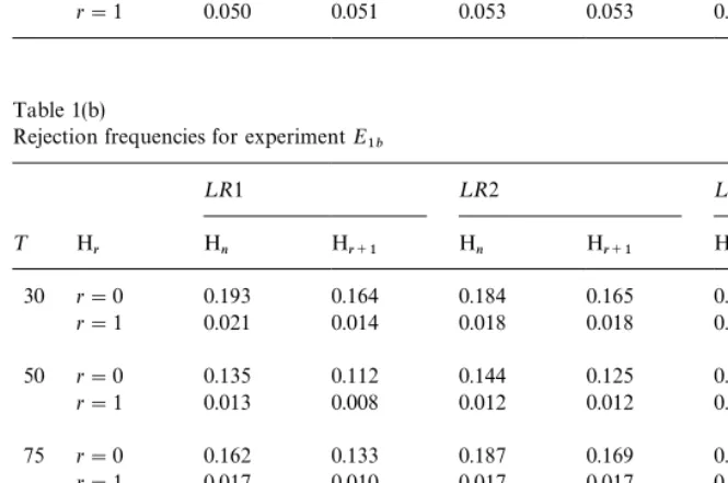
r"0, 1, are summarized in Tables 1(a)}1(d) for the experiments in Set I. The
results in Table 1(a) for ExperimentE
1a show that all tests tend to be
under-sized when¹)150. Because the size distortion is fairly uniform across the tests,
it is possible to directly compare their power properties. The power of the¸R3
tests of Section 5 is signi"cantly higher than their¸R1 and¸R2 counterparts
with the power of the¸R2 tests of Sections 4.1 and 4.2 being slightly better than
the ¸R1 tests of Johansen (1991) in most cases. There seems little to choose
between the¸R3 tests for H
r against Hr`1and Hn although the former test is
slightly more powerful for ¹'50. Similar conclusions may be drawn from
ExperimentE
1b summarized in Table 1(b).
In ExperimentE
1c, see Table 1(c), all tests are slightly over-sized for¹*150.
The¸R3 tests still perform best in terms of power with the¸R2 test also slightly
more powerful than the¸R1 tests. In relative terms, the results are similar to
those in Table 1(a) but the powers of the tests are now signi"cantly greater than
those obtained for ExperimentE
1a. Consequently, a non-zero value fora(which
results in a higher value of the populationR2
*yit,i"1, 2) may improve the"nite
sample power performance of the tests. As above, there is little di!erence
between the results for ExperimentsE
1c andE1d in Tables 1(c) and 1(d),
respec-tively, indicating that the structural error correlation parameterohas little e!ect
on the"nite sample performance of these tests for the experiments in Set I.
Tables 2(a)}2(d) summarize the experiments in Set II. The results in Table 2(a)
for ExperimentE
2a are very similar to those in Tables 1(a) and 1(b). However,
Table 2(b) for ExperimentE
2bindicates that as¹increases all tests, from being
under-sized, become slightly over-sized and then approach nominal size. Unlike
the experiments in Set I, the non-zero value ofo, although it does not result in
Table 1(a)
Rejection frequencies for experimentE
1a
¸R1 ¸R2 ¸R3
¹ H
r Hn Hr`1 Hn Hr`1 Hn Hr`1
30 r"0 0.204 0.166 0.196 0.172 0.265 0.263 r"1 0.024 0.015 0.020 0.020 0.024 0.024 50 r"0 0.151 0.123 0.164 0.140 0.254 0.254 r"1 0.017 0.009 0.015 0.015 0.019 0.019 75 r"0 0.199 0.159 0.226 0.206 0.345 0.352 r"1 0.020 0.013 0.022 0.022 0.025 0.025 100 r"0 0.280 0.248 0.342 0.326 0.475 0.492 r"1 0.029 0.019 0.031 0.031 0.034 0.034 150 r"0 0.418 0.430 0.524 0.549 0.723 0.764 r"1 0.033 0.031 0.040 0.040 0.043 0.043 300 r"0 0.957 0.988 0.988 0.999 0.997 0.999 r"1 0.050 0.051 0.053 0.053 0.053 0.053
Table 1(b)
Rejection frequencies for experimentE
1b
¸R1 ¸R2 ¸R3
¹ H
r Hn Hr`1 Hn Hr`1 Hn Hr`1
30 r"0 0.193 0.164 0.184 0.165 0.304 0.309 r"1 0.021 0.014 0.018 0.018 0.025 0.025 50 r"0 0.135 0.112 0.144 0.125 0.280 0.284 r"1 0.013 0.008 0.012 0.012 0.020 0.020 75 r"0 0.162 0.133 0.187 0.169 0.350 0.356 r"1 0.017 0.010 0.017 0.017 0.025 0.025 100 r"0 0.227 0.196 0.278 0.257 0.461 0.478 r"1 0.022 0.016 0.025 0.025 0.032 0.032 150 r"0 0.419 0.429 0.519 0.547 0.724 0.768 r"1 0.036 0.035 0.036 0.036 0.042 0.042 300 r"0 0.958 0.991 0.989 0.998 0.997 1.00
Table 1(c)
Rejection frequencies for experimentE
1c
¸R1 ¸R2 ¸R3
¹ H
r Hn Hr`1 Hn Hr`1 Hn Hr`1
30 r"0 0.231 0.182 0.221 0.192 0.291 0.279 r"1 0.028 0.019 0.024 0.024 0.029 0.029 50 r"0 0.203 0.159 0.221 0.188 0.323 0.308 r"1 0.024 0.015 0.022 0.022 0.030 0.030 75 r"0 0.299 0.257 0.351 0.329 0.486 0.490 r"1 0.033 0.024 0.034 0.034 0.044 0.044 100 r"0 0.443 0.431 0.535 0.541 0.680 0.707 r"1 0.044 0.036 0.047 0.047 0.055 0.055 150 r"0 0.763 0.824 0.858 0.896 0.934 0.959 r"1 0.054 0.053 0.058 0.058 0.060 0.060
300 r"0 1.00 1.00 1.00 1.00 1.00 1.00
r"1 0.056 0.055 0.057 0.057 0.060 0.060
Table 1(d)
Rejection frequencies for experimentE
1d
¸R1 ¸R2 ¸R3
¹ H
r Hn Hr`1 Hn Hr`1 Hn Hr`1
30 r"0 0.226 0.182 0.219 0.188 0.304 0.309 r"1 0.027 0.017 0.022 0.022 0.025 0.025 50 r"0 0.198 0.157 0.220 0.188 0.351 0.339 r"1 0.023 0.015 0.022 0.022 0.033 0.033 75 r"0 0.289 0.252 0.345 0.322 0.515 0.521 r"1 0.033 0.023 0.036 0.036 0.047 0.047 100 r"0 0.433 0.422 0.526 0.529 0.707 0.734 r"1 0.041 0.033 0.046 0.046 0.060 0.060 150 r"0 0.751 0.811 0.848 0.888 0.946 0.968 r"1 0.054 0.052 0.057 0.057 0.063 0.063
300 r"0 1.00 1.00 1.00 1.00 1.00 1.00
Table 2(a)
Rejection frequencies for experimentE
2a
¸R1 ¸R2 ¸R3
¹ H
r Hn Hr`1 Hn Hr`1 Hn Hr`1
30 r"0 0.202 0.163 0.191 0.169 0.227 0.216 r"1 0.022 0.015 0.018 0.018 0.021 0.021 50 r"0 0.156 0.128 0.166 0.146 0.217 0.201 r"1 0.015 0.009 0.014 0.014 0.019 0.019 75 r"0 0.197 0.164 0.233 0.210 0.295 0.278 r"1 0.021 0.012 0.022 0.022 0.028 0.029 100 r"0 0.276 0.251 0.340 0.332 0.424 0.425 r"1 0.027 0.022 0.029 0.029 0.038 0.038 150 r"0 0.521 0.554 0.642 0.681 0.747 0.796 r"1 0.041 0.036 0.043 0.043 0.050 0.050 300 r"0 0.986 0.998 0.998 1.00 1.00 1.00
r"1 0.054 0.054 0.053 0.053 0.056 0.056
Table 2(b)
Rejection frequencies for experimentE
2b
¸R1 ¸R2 ¸R3
¹ H
r Hn Hr`1 Hn Hr`1 Hn Hr`1
30 r"0 0.258 0.197 0.247 0.211 0.276 0.251 r"1 0.035 0.023 0.028 0.028 0.030 0.030 50 r"0 0.262 0.210 0.291 0.254 0.349 0.323 r"1 0.032 0.021 0.030 0.030 0.038 0.038 75 r"0 0.408 0.377 0.474 0.469 0.559 0.559 r"1 0.047 0.034 0.046 0.046 0.054 0.054 100 r"0 0.597 0.616 0.691 0.718 0.773 0.804 r"1 0.055 0.049 0.055 0.055 0.066 0.066 150 r"0 0.897 0.942 0.951 0.972 0.977 0.989 r"1 0.060 0.057 0.057 0.057 0.060 0.060
300 r"0 1.00 1.00 1.00 1.00 1.00 1.00
Table 2(c)
Rejection frequencies for experimentE
2c
¸R1 ¸R2 ¸R3
¹ H
r Hn Hr`1 Hn Hr`1 Hn Hr`1
30 r"0 0.285 0.209 0.274 0.229 0.348 0.298 r"1 0.044 0.026 0.033 0.033 0.057 0.057 50 r"0 0.324 0.261 0.364 0.325 0.502 0.465 r"1 0.044 0.030 0.042 0.042 0.077 0.077 75 r"0 0.524 0.501 0.600 0.600 0.768 0.781 r"1 0.058 0.047 0.061 0.061 0.096 0.096 100 r"0 0.735 0.769 0.814 0.842 0.932 0.948 r"1 0.066 0.062 0.065 0.065 0.094 0.094 150 r"0 0.965 0.986 0.984 0.993 0.998 0.999 r"1 0.064 0.060 0.060 0.060 0.079 0.079
300 r"0 1.00 1.00 1.00 1.00 1.00 1.00
r"1 0.061 0.060 0.058 0.058 0.066 0.066
Table 2(d)
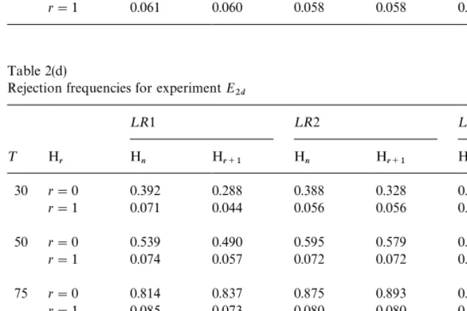
Rejection frequencies for experimentE
2d
¸R1 ¸R2 ¸R3
¹ H
r Hn Hr`1 Hn Hr`1 Hn Hr`1
30 r"0 0.392 0.288 0.388 0.328 0.496 0.435 r"1 0.071 0.044 0.056 0.056 0.093 0.093 50 r"0 0.539 0.490 0.595 0.579 0.770 0.763 r"1 0.074 0.057 0.072 0.072 0.119 0.119 75 r"0 0.814 0.837 0.875 0.893 0.964 0.972 r"1 0.085 0.073 0.080 0.080 0.113 0.113 100 r"0 0.958 0.978 0.978 0.987 0.997 0.998 r"1 0.082 0.078 0.078 0.078 0.103 0.103
150 r"0 1.00 1.00 1.00 1.00 1.00 1.00
r"1 0.068 0.066 0.066 0.066 0.079 0.079
300 r"0 1.00 1.00 1.00 1.00 1.00 1.00
Table 2(c) for ExperimentE
2c demonstrates that the under-size problem of
previous experiments is not a general feature of these tests in small samples.
Both¸R3 tests are now over-sized with the¸R1 and¸R2 tests oversized for
¹)100, for example, the ¸R3 tests have empirical size 0.096 for ¹"75.
Consequently, power comparisons of the di!erent tests are problematic and the
signi"cantly large power of the¸R3 tests over the others'should be discounted.
Subject to this caveat, the comparisons between the tests are quite similar to
those reported earlier. Table 2(d) for ExperimentE
2dreveals similar conclusions.
However, the results for the experiments in Set II tend to be more sensitive to
non-zero-values ofaandothan those for those in Set I.
In summary, the above results suggest that all tests perform reasonably satisfactorily in most of the cases considered. Albeit quite slowly, the empirical sizes of all tests tend to the nominal level as the sample size increases.
Further-more, the¸R3 tests of Section 5 are more powerful than the other tests although
there are situations where these tests tend to over-reject in small samples.
7. An empirical application:A re-examination of the long-run validity of the PPP and UIP hypotheses
In this section we re-examine the empirical evidence on the long-run validity of the Purchasing Power Parity (PPP) and Uncovered Interest Parity (UIP) hypotheses presented in Johansen and Juselius (1992) and Pesaran and Shin (1996). In these applications domestic and foreign prices and interest rates are assumed to be endogenously determined. Such a symmetric treatment of domes-tic and foreign variables does not, however, seem to be necessary in the case of small open economies where it is unlikely that changes in domestic variables
have a signi"cant impact on the long-run evolution of foreign (world) prices or
interest rates. This earlier analysis also included changes in the logarithm of oil
prices and its lagged values as exogenous I(0) variables in the underlying
cointegrating VAR model. However, as discussed in Section 4.3, the appropriate
method of allowing for such e!ects is to include an integrated version of theI(0)
variables in the model which, in the context of the present application, implies
adding the logarithm of oil prices to the list ofI(1) variables, and then testing the
validity of excluding the level of oil prices from the cointegrating relations. For comparability purposes, we use the same quarterly observations em-ployed by Johansen and Juselius. The data set relates to the U.K. economy and
covers the period 1972(1)}1987(2). The includedI(1) variables are: the logarithm
of the e!ective exchange rate,e
t, the logarithm of the U.K. wholesale price index,
p
t, the logarithm of the trade-weighted foreign wholesale price index, pHt, the
logarithm of oil prices,po
t, and the domestic and foreign interest rate variables,
r
t"ln (1#Rt/100) andrHt"ln (1#RHt/100), whereRtis the U.K. three-month
20These results are based on the assumption that pHard po areI(1) and non-cointegrated. However, it is possible to test this assumption (see Theorems 4.7 and 4.8). Using an unrestricted trend VAR(3) model in these exogenous variables, augmented with two lagged changes in the endogenous variables we could not reject the hypothesis thatpHandpoare non-cointegrated. The choice of the order of the VAR in this application was based on the Schwarz Bayesian Criterion and the choice of trend speci"cation was based on the speci"cation test of Theorem 4.5.
a cointegration analysis on the sixI(1) variables,e
t,pt,rt,rHt,pHt, andpot, treating the last two variables as weakly exogenous and, thus, long-run forcing, in the sense described in Section 3. We also considered treating the foreign interest rate
variable rH
t as exogenous but, given the importance of the U.K. in world
"nancial markets, it was felt that this was unlikely to be justi"ed.
Consequently, the appropriate framework for this application is the model de"ned by (3.5) and (3.6). Following Johansen and Juselius (1992) we setp"2
but did not include seasonal dummies in the model. The seasonal e!ects were
only marginally signi"cant and given the limited sample size available it was
thought best to leave them out. With the foreign price and oil price variables,
pHt andpo
t, treated asI(1) and exogenous, we estimated the following system of
equations over the period 1972(3)}1987(2):
*y
coe$cient matrices, and K a (4,2) coe$cient matrix. Note that in the above
speci"cation the trend coe$cients (!P
yc) are restricted as in Case IV de"ned
by (3.12) and, hence, the level ofy
twill exhibit linear deterministic trends for all
values of the cointegration rankr"Rank(P
y). These restrictions on the trend
coe$cients can be tested using standard chi-squared tests set out in Theorem
4.5. The (log-) likelihood ratio statistics for testing the trend restrictions (Case
IV) against the unrestricted trend speci"cation (Case V) for r"0, 1, 2, 3 are
7.61[9.49], 7.26[7.81], 4.73[5.99], and 2.24[3.84], respectively. The"gures in [.]
are the 0.05 critical values of the chi-squared distribution with 4!rdegrees of
freedom. Therefore, irrespective of the value ofrthe trend restrictions cannot be
rejected.
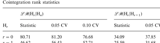
Table 3 reports the cointegration rank test statistics de"ned byLR(H
rDHn)
andLR(H
rDHr`1) of (4.7) and (4.5) respectively, together with the
correspond-ing asymptotic critical values at the 0.05 and 0.10 signi"cance levels reproduced
from Table 6(d) withk"2 andn!r"4, 3, 2, 1.
Neither statistic rejects the hypothesis of no cointegration at the 0.05 signi"
-cance level but LR(H
rDHn) rejects the null of no cointegration at the 0.10
level.20If we con"ned our analysis solely to these statistical tests, we could only
conclude that there is at mostone cointegrating relation between the six I(1)
Table 3
Cointegration rank statistics
LR(H
rDHn) LR(HrDHr`1)
H
r Statistic 0.05 CV 0.10 CV Statistic 0.05 CV 0.10 CV
r"0 80.71 81.20 76.68 34.09 37.85 35.04 r"1 46.62 56.43 52.71 25.59 31.68 29.00 r"2 21.03 35.37 32.51 14.10 24.88 22.53
r"3 6.93 18.08 15.82 6.93 18.08 15.82
However, economic theory suggests the existence of two long-run
(cointegrat-ing) relations in the above system, namely the PPP and UIP relations de"ned as
p
t!et!pHt andrt!rHt, respectively. Since in this application the sample size is
relatively small (¹"60) and the dimension of the system is relatively large
(m"6), the evidence against the hypothesis of two cointegrating relations does not seem to be particularly strong. Moreover, the Monte Carlo simulation results of Section 6 indicate that these cointegrating rank test statistics generally tend to under-reject in small samples. We therefore examine the case in which restrictions on short-run dynamics are available and are imposed in the con-struction of the (log-) likelihood ratio tests of the cointegrating rank restrictions;
see Section 5. A preliminary analysis of the regressions for*p
t,*et,*rtand*rHt
suggest the following 24 zero restrictions on the short-run coe$cients:
K"
C
0 *
0 0
0 0
0 0
D
, W
1"
C
* 0 0 0 0 0
0 * * 0 0 *
0 0 * 0 0 0
0 0 0 * * 0
D
, (7.2)
where unrestricted coe$cients are denoted by*. The maximized log-likelihood
values of the restricted and the unrestricted model together with the associated Akaike Information Criterion (AIC) and the Schwarz Bayesian Criterion (SBC) are given by
Unrestricted Restricted
LL 725.01 716.49
AIC 661.01 676.49
SBC 593.99 634.61
Table 4
Cointegration rank statistics for short-run restricted model
LR'C(H
rDHn) LR
'C(H
rDHr`1)
H
0 Statistic 0.05 CV 0.10 CV Statistic 0.05 CV 0.10 CV
r"0 139.62 81.20 76.68 75.73 37.85 35.04 r"1 63.89 56.43 52.71 37.08 31.68 29.00 r"2 26.80 35.37 32.51 19.60 24.88 22.53
r"3 7.21 18.08 15.82 7.21 18.08 15.82
Table 4 reports the cointegration rank statistics LR'C(H
rDHn) and
LR'C(H
rDHr`1) of Section 5 based on the above restricted model.
These statistics do not reject the null hypothesis ofr"2 which is in line with
the prediction of economic theory. Consequently, we proceed as if there are two co-integrating relations. We return subsequently to re-consider the case of
cointegrating rankr"1 to see the extent to which our conclusions based on
r"2 regarding the long-run validity of the PPP hypothesis are a!ected by this choice ofr.
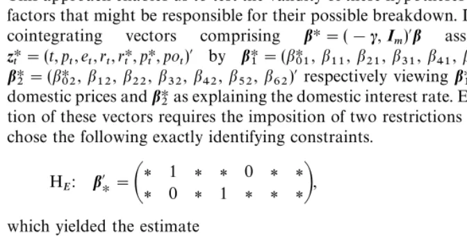
We now examine the validity of the PPP and UIP hypotheses using the long-run structural modelling techniques advanced in Pesaran and Shin (1999). This approach enables us to test the validity of these hypotheses and to identify factors that might be responsible for their possible breakdown. Denote the two
cointegrating vectors comprising bH"(!c, I
m)@b associated with
zHt"(t,p
t,et,rt,rHt,pHt,pot)@ by bH1"(bH01,b11, b21, b31, b41,b51, b61)@ and
bH2"(bH02, b12,b22, b32, b42, b52,b62)@ respectively viewingbH1 as explaining
domestic prices andbH2as explaining the domestic interest rate. Exact identi" ca-tion of these vectors requires the imposica-tion of two restricca-tions per vector. We chose the following exactly identifying constraints.
H
E: b@H"
A
*1 * * 0 * *
* 0 * 1 * * *
B
,which yielded the estimate
bK@ HE"
A
0.0195 1 !0.701 !6.005 0 !2.564 0.206(0.0229) (0.345) (2.088) (1.943) (0.274)
!0.0062 0 !0.091 1 !0.791 0.493 !0.054
(0.0038) (0.095) (0.326) (0.334) (0.046)
B
,
¸¸
21All the computations reported in this section are carried out usingMicroxt4.0. See Pesaran and Pesaran (1997).
22Recall that the primary motivation behind the inclusion of oil prices in this model is to capture the short-run e!ects of changes in oil prices on the PPP and the UIP relations.
where¸¸
E is the maximized value of the log-likelihood function for the
just-identi"ed case. Asymptotic standard errors are given in parentheses.21
A number of hypotheses of interest may now be tested using the above exactly identi"ed model. Consider"rstly the co-trending hypothesis H
#0, namely that
the trend coe$cients are zero in the two cointegrating relations:
H
#0: b@H"
A
0 1 * * 0 * *
0 0 * 1 * * *
B
,Under H
#0, we obtained the estimate
bK@ H#0"
A
0 1 !0.881 !5.511 0 !0.854 !0.025
(0.333) (1.748) !(0.280) (0.048)
0 0 !0.037 1 !0.929 !0.067 0.023
(0.101) (0.414) (0.053) (0.015)
B
,
¸¸
#0"713.30.
Therefore, the log-likelihood ratio statistic for testing the co-trending hypothesis
is equal to 2(714.50}713.30)"2.40, which is below the 0.05 critical value of the
chi-squared distribution with 2 degrees of freedom. Hence, the co-trending hypothesis is not rejected.
We now consider the hypothesis that level of oil prices do not enter the cointegrating relations which we denote by H
10.22To save space, we only report
the test of this hypothesis jointly with the co-trending hypothesis, H
#0WH10,
which yields
bK@
H#0,10"
A
0 1 !0.834 !5.646 0 !0.925 0
(0.327) (1.850) (0.227)
0 0 !0.062 1 !0.803 !0.005 0
(0.129) (0.432) (0.063)
B
,
¸¸