Adaptive information processing in microtubule networks
Jeffrey O. Pfaffmann, Michael Conrad *
Department of Computer Science,Wayne State Uni6ersity,Detroit,MI48202,USA
Abstract
Microtubule networks provide a wide range of microskeletal and micromuscular functionalities. Evidence from a number of directions suggests that they can also serve as a medium for intracellular signaling processing. The model presented here comprises an empirically motivated representation of microtubule growth dynamics, an abstract representation of signal processing, and a feedback learning mechanism that we refer to as adaptive self-stabilization. The growth model mimics the dynamic instability picture of microtubule formation and decomposition, but as modulated by the binding activity of microtubule associated proteins (or MAPs). The signal processing submodel treats each microtubule as a string of linked discrete oscillators capable of propagating signals that are introduced, manipulated, and extracted by bound MAP activity. Adaptive self-stabilization is essentially feedback acting on signal processing capabilities via the growth dynamics. The network is presented with a training set of patterns. If the input – output behavior is satisfactory MAP binding affinity increases, thereby stabilizing the network structure; otherwise the binding affinity decreases, allowing for more structural variation. The results obtained suggest that adaptive capabilities are practically inevitable in microtubule networks, a conclusion strengthened by the fact that the signal processing and growth dynamics mechanisms available in nature are undoubtedly much richer than those represented in the model. © 2000 Elsevier Science Ireland Ltd. All rights reserved.
Keywords:Microtubule signal processing; Adaptive self-stabilization; Dynamic instability; Adaptive information processing www.elsevier.com/locate/biosystems
1. Introduction
Microtubules are polymacromolecular fibers that are instrumental in a wide variety of pro-cesses in eucaryotic cells: mitosis, axonal trans-port, organelle organization and more generally for structural integrity and dynamic form. The specific functions performed depend on auxiliary proteins (microtubule associated proteins, or MAPs for short) that strongly influence the
struc-ture of the fibrous network and its interactions with membranes and other components of the cytomatrix (Matus, 1988). It is likely that micro-tubules also provide a medium for long range intracellular signaling (Kirkpatrick, 1979; Mat-sumoto and Sakai, 1979; Liberman et al., 1982, 1985; Hameroff and Watt, 1982; Hameroff, 1987; Conrad, 1991). Various adaptation mechanisms have also been proposed (Conrad et al., 1989; Conrad, 1990; Rasmussen et al., 1990; Chen and Conrad, 1994; Ugur and Conrad, 1997). Adapta-tion on a phylogenetic time scale could easily occur through population based variation and * Corresponding author.
E-mail address:[email protected] (M. Conrad)
selection acting on MAPs. The question addressed here is whether learning can occur on an individ-ual cell level within a single life cycle.
The model to be presented combines an empiri-cally motivated growth mechanism with a general but abstract representation of signal processing. The growth mechanism implements the low level dynamics of microtubule assembly to simulate what is sometimes referred to as dynamic instabil-ity (Wordeman and Mitchison, 1994). This term refers to the fact that the net mass of the micro-tubule population can be relatively constant de-spite continual assembly and disassembly of individual microtubules. Here we view dynamic instability as a stochastic search mechanism that modifies the signal processing. The search can continue, in a more fine tuned fashion, even if microtubule assembly and disassembly is frozen, since MAP bindings can still change. Representa-tion of signal processing is more problematic. Many modes are possible, and could even co-ex-ist; but the experimental situation is unclear.
Our choice is to treat the microtubules as strings of coupled oscillators (on a discrete time scale) and to allow MAPs to link the oscillations in neighboring microtubules. The vibratory (or wave) dynamics serves to combine input signals in space and time. Input signals are introduced by readin MAPS, combined in space and time by the vibratory dynamics of the microtubules, and ex-tracted by readout MAPs. Linker and modulating MAPs serve to tune the vibratory dynamics. The coupled oscillator representation can be thought of as a highly simplified field model that could be particularized to a wide variety of specific mecha-nisms. For the present purposes the important point is that the microtubule network serves as a medium of signal integration.
The growth dynamics and signal processing are coupled by a learning mechanism to be referred to as adaptive self-stabilization. The term is intended to suggest negative feedback acting on structure and through this on the signal processing perfor-mance. A microtubule network is first generated by the growth dynamics. The information pro-cessing capabilities of the network are then evalu-ated relative to a training set of patterns. The growth parameters are changed in a manner that
depends on performance. If the network performs well only a small amount of microtubule growth or variation in MAP distribution is allowed. If it performs poorly then the structure is allowed to be more dynamic, commensurate with the fact that the error signal should be greater. The MAP binding affinity in a sense plays the role of tem-perature in simulated annealing; increase and de-crease in binding affinity corresponds to inde-crease and decrease in temperature. When the system reaches an adequate level of learning the micro-tubule structure is frozen. Further learning relies on variations in MAP distribution that would in principle occur through diffusional search.
2. Microtubule biology
Microtubule networks underlie the external (plasma) membrane and extend through the cy-tomatrix in nearly all eucaryotic cells. They are particularly prolific in neurons, where they play an important role (with the aid of MAPs) in the formation and function of both axonal and den-dritic projections (Burgoyne, 1991; Alberts et al., 1994). The individual microtubules are assembled from smaller proteins (tubulin dimers). Network structures are molded by the assembly process and also by a microtubule organizing center (MTOC), influences exerted by bound MAPS, and environmental regulators. The assembly pro-cedure is unique: microtubules can grow by adding new tubulin dimers to a particular end and shrink by reversing this process.
cap on a disassembling microtubule (called res-cue) allows the structure to return to the assembly mode. The dynamic instability phenomenon dis-cussed previously follows from the interplay of cap disappearance and rescue. In the cell the MTOC adds an additional level of organization to dynamic instability by anchoring the non-growth end of the microtubules and thereby ori-enting the growth of the microtubule population as a whole. MAP interactions mold the popula-tion into different configurapopula-tions by stabilizing individual microtubules and by subserving a vari-ety of other organizational roles.
The growth dynamics described above provide four points of regulation. The first is the number of dimers that are converted from straight to curved in the lateral cap. This regulates the assem-bly characteristics of the individual microtubules. Second is the number of free dimers that can be incorporated into microtubules. Regulation of the binding efficiency of structure stabilizing MAPs is the third. The characteristics of the MAPs them-selves afford the fourth point of regulation. MAPs constitute a large family of proteins. Alterations in the MAP population can thus influence net-work organization and functionality. These possi-bilities for regulation suggest that microtubule networks are moldable systems that can develop into a variety of configurations capable of per-forming different tasks.
3. Model specification
3.1. O6er6iew
We picture the microtubule network as embed-ded in a section of the intra-neuronal environ-ment, represented in terms of a three dimensional array (Fig. 2). Each location in the array is a cube of specified size, indexed in the figure by jkl. The cube size controls the amount of total protein mass, including MAP as well as microtubule mass, that can occupy the location. The amount allowed is measured in units of 100 kDa, or the mass of one tubulin dimer (called a dimer unit). One kDa is equivalent to the mass of 1000 hydro-gen atoms.
Microtubules exclusively occupy one or more contiguous array locations along the l-axis. Each array location is considered to contain a separate subregion of the microtubule comprising 60 dimers (or fewer in the case of the growing tip). This corresponds to a cube edge of 37 nm. The restriction to one direction of growth results in a population of parallel (but potentially interlinked) microtubules similar to natural networks regu-lated by MTOC and MAP organizational effects. MAPs are represented as independent data structures that diffuse in the array, implemented Fig. 1. Role of lateral cap in microtubule assembly and
disassembly. The conformational state of assembled dimers may be either straight or curved. Straight dimers favor assem-bly (black ovals). Curved dimers favor disassemassem-bly (white ovals).
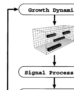
Fig. 3. Cyclic flow of control. The growth dynamics and signal processing modules share a common microtubule network representation (see Fig. 2). The adaptive self-stabilization module couples the growth dynamics to signal processing performance.
defined training set. Desired outputs are assigned to the input patterns used for training.
The growth module is modified by changing MAP binding affinity and by freezing the micro-tubule assembly process at a particular learning level (at which point learning proceeds only through MAP diffusion). Increasing the binding affinity increases network stability, while decreas-ing the affinity decreases stability. When the net-work performs well binding affinity is increased. The extent of structure change accordingly de-creases. If the network performs poorly binding affinity decreases, allowing for increased structure change. Freezing the growth process at a certain learning level protects the network structure from the erratic effects of growth on the signal process-ing dynamics.
3.2. Growth dynamics
The growth module creates a population of dynamic individuals that exhibit a net stability. The dynamics are based on empirical evidence for a lateral cap (Timasheff, 1991) and computer simulation of cap dynamics in vitro (Bayley et al., 1994). However, our model, as currently formu-lated, does not attempt to match the growth rates of the natural system.
The following three factors must be taken into account: available straight dimers, dimers bound in microtubules, and lateral cap size. The pool of available straight dimers at time t, to be denoted by A(t), is treated as homogeneously distributed throughout the intracellular environment. The pool size at time t+1 given by
A(t+1)=A(t)−G(t)
+dempty array locations at time t
total array locations (1)
where G(t) is the number of dimers incorporated in the microtubule network at time tanddis the maximum number of dimers that can be added at each time step (to be referred to as the new dimer coefficient). The ratio of empty array locations to total locations thus serves as a low-level feedback mechanism ensuring that a consistent mass is maintained.
by stochastically moving the data structure from one array location to another. MAPs can be in either a bound or free state. Bound MAPs are part of the microtubule network and influence its dynamics. Accordingly they are not allowed to diffuse when in this state. Free MAPs are not part of the network, exerting no influence on it, and thus are allowed to diffuse. Five different MAP types will shortly be introduced. Each MAP type can consist of subtypes with a unique set of characteristics.
pre-Let gn(t) represent the number of straight dimers incorporated into microtubulen at timet. This is taken as a random value from 1 to 60.
G(t) is then the sum of thegn(t). The size of the lateral cap of microtubule n at time t+1, to be denoted bycn(t+1), is given by
cn(t+1)=
!
L if L]0
0 otherwise (2)
whereL=cn(t)+gn(t)–ris the lateral cap size at
timet, andris the number of dimers hydrolyzed, to be referred to as the hydrolysis coefficient.
The above three factors determine the number of array locations a microtubule will occupy, i.e. how many subregions the microtubule is divided into (Fig. 2). For every 60 dimers added the microtubule will increase by one subregion. This size increase respects array locations currently occupied by other microtubules and also respects array boundaries. The important point is that each array location represents a segment of the microtubule, not an individual dimer. This choice is for computational convenience. Decreasing the number of dimers associated with an array loca-tion would yield a more refined descriploca-tion; but the computational resources allocated to the rep-resentation must be balanced against the compu-tational resources required for the learning process.
If the lateral cap should disappear (i.e. if
cn(t)=0) the microtubule will lose one subregion at each time stept(unless a bound MAP prevents disassembly). Rescue, which switches micro-tubules from shrinking to growth, is implemented by randomly generating a value for gn(t), the number of straight dimers to be incorporated, and then comparing this to the hydrolysis coefficient (r). If the number of added dimers is greater than
the hydrolysis coefficient (i.e. the number of dimers lost) the lateral cap re-forms and the mi-crotubule resumes growing.
Typical growth behavior is illustrated in Fig. 4. This shows the percentage of the space occupied by three different microtubule populations. MAPs were not present in any of these cases. The only difference is in the hydrolysis coefficient (r). As can be seen, the total microtubule mass is in-versely proportional to the hydrolysis coefficient. The dimer coefficient (d) has a directly propor-tional effect (not shown here).
The stabilizing effect of bound MAPs on the growth dynamics is effectuated by preventing dis-assembly of the subregion to which they are bound. Unbound (or free) MAPs are stochasti-cally rearranged, as would happen in a diffusive process. This is implemented by moving the MAP one array location in a random direction at each time step t. MAP movement is restricted in two ways: MAPs cannot leave the array space and they can only move into an array location if the mass restriction will not be violated.
3.3. Signal processing
After the growth dynamics module has com-pleted its work for a given iteration the signal processing module takes over. Each microtubule is now treated as a string of coupled oscillators, in the fashion of a loaded string (Marion and Thornton, 1995), except that the time develop-ment is discretized (Boole, 1958). The string is divided into masses connected by springs with each mass representing a microtubule subregion and the springs representing the collective dimer binding forces. A given mass on the string of oscillators represents sixty dimers (except possibly at the growing tip) and also attached MAPs. As noted in the previous subsection, this lumping increases the computational resources available for the adaptation experiments. The physical cor-respondence between a discretized loaded string and the continuous picture implied by lumping is clearly imperfect, since adjacent subregions of the microtubule are as close to each other as the dimers within these subregions. But for the Fig. 4. Time variation of a microtubule network size for three
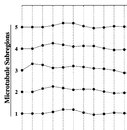
Fig. 5. Signal propagation dynamics of a single microtubule containing five subregions. The graph should be read from left to right, with each time step indicating the state of the microtubule at that time. Thus the displacements from the equilibrium position represent longitudinal motions in the vertical direction.
MAPs), K is the spring constant, o is a damping coefficient representing energy lost to the environ-ment, and Bjkl(t) is the total displacement due to energy introduced due to active MAP effects. The boundary conditions are set by eliminating the terms containing xjk(l+1) and xjk(l−1) (for the left
and right string boundaries, respectively). Thus we view the string as pinned at both ends.
The vibrations are longitudinal if Kis taken as a spring constant, as above. The same equation describes transverse oscillations if Kis interpreted as the tension in the string divided by intermass spacing (Marion and Thornton, 1995). The longi-tudinal picture is more natural here, since the separation of the microtubule into different subre-gions is rather arbitrary. Fig. 5 illustrates the longitudinal oscillatory behavior of a microtubule containing five subregions. The parameters used to generate this figure are a total mass (M) corre-sponding to 6000 kDa for each subregion, a unit time scale spring constant (K) of 3000 kDa, and a unit time scale damping coefficient (o) of 1000 kDa (recognizing that the dimensions are not biophysically meaningful, due to the discretization of time). The figure shows that the system is at rest at t=0, then at t=1 energy is added to subregion 3 in the form of a mass displacement. From that point on one can see the wave propa-gating through the structure. Note that nothing prevents the masses from passing through each other given the potential function used, apart from an appropriate choice of parameters. Also, a negative value of o can be used to represent pumping of energy into the network in response to its oscillatory activity, hence a nonspecific form of amplification.
Adding bound MAPs would have the passive effect of increasing subregion mass and reducing the oscillatory activity. There are also a number of ways in which MAPs, when triggered, can introduce energy into the subregion of the micro-tubule to which they are bound, thereby causing displacement of that subregion. The energy re-lease is here pictured in mechanochemical terms. Five different MAP types play a role (readin, readout, linkers, amplifiers, and modulators). Readin MAPs are used to introduce a pattern into the network. Readout MAPs extract signals from present purposes it is sufficient for the signal
processing module to provide a variety of wave-like behaviors that serve to combine signals in space and time in a way that depends on the structure of the network.
Let xjkl(t) represent the position of the mass associated with array locationjklat timetrelative to its position at rest (xjkl(t)=0). The timethere is distinct from the time t used by the growth module. This time development is described by
xjkl(t+1)=2xjkl(t)−xjkl(t−1)
+ K
Mjkl
[xjk(l+1)(t)−2xjkl(t)
+xjk(l−1)(t)]
+ o
Mjkl
[xjkl(t−1)−xjkl(t)]+Bjkl(t)
(3)
where the time increment is set equal to unity.
the microtubule network. Linker MAPs are trig-gered by the vibratory activity of a microtubule in a neighboring array location. Amplifier MAPs respond to the vibratory activity of the location to which they are bound. Modulators contribute pas-sive effects to the signal process by increasing mass. The linker and amplifier maps introduce the essen-tial nonlinearities into the network dynamics.
The total mass displacement,Bjkt(t), effected by MAP active effects at locationjkl, is the sum of all displacements produced by readins, linkers, and amplifiers. To release energy into a subregion, these MAPs must first be triggered. Readin MAPs are automatically triggered to introduce signals into the network. For linkers and amplifiers the assumption is that they are change detectors that respond to the change in velocity of a specific subregion. Amplifiers are triggered locally on the subregion to which they are bound. Linkers are slightly more complex because they are triggered by a subregion of a neighboring microtubule (indi-cated by index j%k%l%). The mass displacement
HereDjklwis the mass displacement when the MAP
wtriggers andTjklw, is the value at which MAPw at jkl will trigger when compared to the rate of change at locationj%k%l%. This is determined when the MAP binds to the subregion, as is the location
j%k%l% it detects. The direction of the displacement produced by a MAP is randomly assigned at time of binding. The array location j%k%l% to which it responds is also randomly selected from the 24 possible locations that it could potentially contact.
3.4. Adapti6e self-stabilization
Recall that adaptive self-stabilization is essen-tially error feedback acting on the structure of the microtubule network and on the distribution of MAPs in a given structure. Picture the microtubule networks as immersed in a broadcast cocktail of
biochemical signals that activate a pattern of readin MAPs in a way that depends on their specificities. The signals are combined in space and time by the vibratory dynamics of the network. Readout MAPs may or may not be activated. The error signal depends on the extent to which the consequent outputs are suitable or unsuitable to the environment. The more the error the greater the structural variation exhibited by the network. Adaptive self-stabilization can be thought of as a special case of variation-selection learning, but without a population of reproducing systems for selection to act on.
As previously noted, the extent of network variation is controlled by the binding affinity of the MAPs. If the signal processing performance of the network is good the MAPs will adhere to the microtubule surface strongly, thereby increasing the stability of the network structure. If the perfor-mance is poor the binding to the surface is weak-ened.
Performance is determined relative to a predeter-mined training set. This consists of a set of input patterns and a desired output (1 or 0). The training set is processed (on time scalet) after each growth cycle iteration (on time scalet). The signal process-ing is successful if it produces a 1 output within a required amount of time for each input pattern that calls for this output and produces no output during this time period if the input pattern calls for a 0 output. The performance on the training set as a whole is determined by the percentage of correct responses. The binding affinity increases with this percentage (with increasing slope).
search is necessary to give direction to the learning process. In an individual-based model (as opposed to one that uses populations) variations will have increasingly negative effects as the performance increases and especially so for a randomly con-structed task such as the one used here. Some memory mechanism is necessary that allows the system to return to a previous state if the variation has destructive effects. The fitness function would not otherwise provide direction by selecting better variations; it would only control the extent to which the microtubules and MAP distribution are shaken.
4. Learning results
The signal processing capabilities of the model were tested using three randomly generated train-ing sets. Each traintrain-ing set consisted of binary input patterns of fixed size: 4-bit, 5-bit, and 6-bit. All possible combinations of input patterns are repre-sented in each training set. Thus the 6 bit set contained 64 instances (26 patterns). A single
out-put bit was randomly assigned to each inout-put pattern, resulting in an approximately 50% split of the training set between the two subsets. The purpose was to test the model’s capacity to learn associations under the most difficult conditions, namely the absence of any structure in the training set. The issue of generalization has not at this point been addressed. Training sets without any struc-ture (i.e. without any similarity among input pat-terns that should be classified the same way) actually afford no possibility for sensible general-ization (Ugur and Conrad, 1997).
Each of the three training sets was tested by varying the hydrolysis coefficient to give different microtubule densitites and run with 20 different random seed values, producing 60 program runs per training set. The program runs were broken into groups of 20 (but with the hydrolysis coeffi-cient held constant within each group). The net-work was required to respond within 7 time steps on the signal processing time scale which was sufficiently long for signals to propagate through the network.
Fig. 6 shows the average performance for a
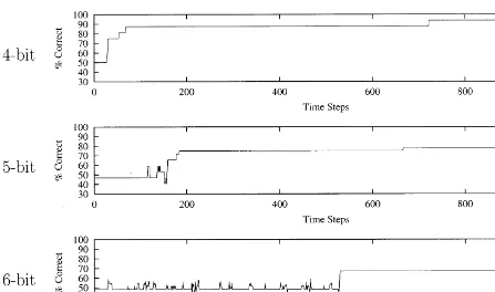
single group or runs for each training set for 1000 growth cycles (using the group whose hydrolysis coefficients yield the best average performance). The 4-bit group reached the 76% learning level; the 5- and 6-bit groups hit averages of 70 and 63%, respectively. Within each group there are individu-als that achieved a reasonably good performance (see Fig. 7). The best individual in the 4-bit training group reached 94% at the time of termination. The 5-bit training group included 11 individuals (out of 20) that exceeded 70%, with the best reaching 78%. The 6-bit group included only one individual that reached the 70% level.
As expected, the performance decreased as the size of the training patterns increased, correspond-ing to the combinatorial increase in the difficulty of pattern recognition problems. This is reflected in the fact that the 4- and 5-bit cases were frozen at the 65% level of learning, whereas the 6-bit case was frozen at the 60% level in the data reported. The chance of randomly reaching a pre-specified freezing level decreases as the problem size in-creases, due to the fact that the number of patterns that must be recognized correctly increases.
slope (as in the runs reported) the jumpiness increases the chance of finding better solutions, but at the expense of a greater chance of losing these solutions during the periods of exploration. However, once freezing occurs and gradient search is initiated only improvements are retained. This also, of course, restricts the exploratory search.
The results reported in this section give a gen-eral impression of the behaviors observed. The system as currently constituted exhibits learning despite the crudeness of the learning algorithm. Using different binding affinity curves for the different MAP types, depending on how critical they are for integration of signals in space and time, should be an important refinement. The microtubule structure provides the main data pathways; if learning nears stagnation at an inad-equate level these should be allowed to depoly-merize and regrow into a new structure. This was not allowed in the present implementation.
5. Conclusion
Whether microtubule networks in actual bio-logical cells serve as a medium for adaptive infor-mation processing is open from the experimental point of view. The model presented here suggests that it would be hard for them not to do so. All that is necessary is a coupling of fast dynamics that serves to combine influences in space and time with the slow dynamics of growth and MAP redistribution. The simplifying assumptions of the model actually strengthen this conclusion. The much richer biological reality affords multiple possibilities for propagation and processing of impinging influences (referred to in the model as signal processing). The growth process and con-trols over MAP distribution are clearly more elab-orate in cells than is represented in the model. It would be difficult to decouple these morphologi-cal aspects from the signal processing aspect. Ac-tions unsuited to the environmental situation
Fig. 6. Average learning curves for 20 runs from a group with different random seed values. The 4-bit growth parameters were
Fig. 7. Best learning curves from 20 runs from a group with different random seed values. The 4-bit growth parameters werer=10 andd=100; 5-bit growth parameters werer=10 andd=100; 6-bit growth parameters werer=5 andd=100.
Fig. 8. Learning curves showing effects of MAP alteration without freezing network growth. The 6-bit growth parameters were
r=10 andd=100 in both cases. The slope of the binding affinity curve increased in the case of (a) and decreased in the case of (b).
follow ineffective signal processing. Adaptive self-stabilization is in a rough way nascent in the infeasibility of isolating the form of the
Has this nascency been developed in the course of evolution into a sophisticated adaptation al-gorithm, or has it been suppressed? Mechanisms more sophisticated than those represented in our model are certainly possible. One possible direc-tion of improvement should in particular be noted. The algorithm used in the present study varied the binding affinities that controlled the integrative dynamics at the same time that it varied the locations of the readouts. In actual biological cells the gross network structure and the distribution of amplifying and linking MAPs would presumably be largely determined by the long process of phylogenetic evolution. The start-ing point for ontogenetic cellular adaptation would be an inherited network structure that is plausibly sufficiently complex for different poten-tial readout locations to be activated by different groupings of input patterns. The readouts could then be added and deleted without interfering with the integrative dynamics, thereby adding and deleting particular input patterns from the set that readouts in other locations respond to. This sepa-ration of integrative and interpretative dynamics, referred to as the principle of double dynamics (Conrad, 1985), would be a further step in the direction of protecting the network from varia-tions that could substantially interfere with previ-ously acquired capabilities.
The microtubule system in vivo is intimately interconnected with the cell membrane and with other fibrous components of the cytoskeleton. Needless to say this further enriches the possibili-ties for coupling signal processing and growth dynamics to achieve self-stabilization learning. From one point of view this means that the model presented here is even simpler relative to the much greater richness of biological cells. But in line with the above it further strengthens the major conclu-sion: the fine structure of the cell is a natural medium for adaptive information processing.
Acknowledgements
This research was supported by the National Science Foundation under Grants ECS-9404190 and EIA-9729818, and by the Fetzer Institute
(through the University of Arizona Consciousness Studies Research Program). Discussions with members of the Wayne State University Biocom-puting Group are gratefully acknowledged.
References
Alberts, B., Bray, D., Lewis, J., Raff, M., Roberts, K., Wat-son, J.D., 1994. Molecular Biology of the Cell. Garland Publishing, Inc, New York.
Bayley, P.M., Sharma, K.K., Martin, S.R., 1994. Microtubule dynamics in vitro. In: Hyams, J., Lloyd, C. (Eds.), Micro-tubules. Wiley-Liss, Inc, New York, pp. 111 – 137. Boole, G., 1958. Calculus of Finite Differences. Chelsea
Pub-lishing Company, New York.
Burgoyne, R.D., 1991. High molecular weight microtubule-as-sociated proteins of the brain. In: Burgoyne, R.D. (Ed.), The Neuronal Cytoskeleton. WileyLiss, Inc, New York, pp. 75 – 91.
Chen, J.C., Conrad, M., 1994. Learning synergy in a multilevel neuronal architecture. Biosystems 32, 111 – 142.
Conrad, M., 1985. On design principles for a molecular com-puter. Comm. ACM 28, 464 – 480.
Conrad, M., 1990. Molecular computing. In: Yovits, M.C. (Ed.), Advances in Computers. Academic Press, San Diego, pp. 236 – 324.
Conrad, M., 1991. Electronic instabilities in biological infor-mation processing. In: Lazarev, P. (Ed.), Molecular Elec-tronics. Kluwer Academic Publishers, Dordrecht, pp. 41 – 50.
Conrad, M., Kampfner, R.R., Kirby, K.G., Rizki, E.N., Schleis, G., Smalz, R., Trenary, R., 1989. Towards an artificial brain. Biosystems 23, 175 – 218.
Hameroff, S.R., Watt, R.C., 1982. Information processing in microtubules. J Theor. Biol. 98, 549 – 561.
Hameroff, S.R., 1987. Ultimate Computing. Elsevier Science Publishers B.V, Amsterdam.
Kirkpatrick, F.H., 1979. New models of cellular control: mem-brane cytoskeletons, memmem-brane curvature potential, and possible interactions. Biosystems 11, 93 – 109.
Liberman, E.A., Minina, S.V., Shklovsky-Kordy, N.E., Con-rad, M., 1982. Change of mechanical parameters as a possible means for information processing by the neuron (in Russian). Biofizika 27, 863 – 870.
Liberman, E.A., Minina, S.V., Mjakotina, O.L., Shklovsky-Kordy, N.E., Conrad, M., 1985. Neuron generator poten-tials evoked by intracellular injection of cyclic nucleotides and mechanical distension. Brain Res. 338, 33 – 44. Marion, J., Thornton, S., 1995. Classical Dynamics of
Parti-cles and Systems. Harcourt Brace & Company, Fort Worth.
Matus, A., 1988. Microtubule-associated proteins: their poten-tial role in determining neuronal morphology. Annu. Rev. Neurosci. 11, 29 – 44.
Rasmussen, S., Karampurwala, H., Vaidyanath, R., Jensen, K., Hameroff, S., 1990. Computational connectionism within neurons: a model of cytoskeletal automata subserving neu-ral networks. Physica D 42, 428 – 449.
Timasheff, S.N., 1991. The role of double rings in the tubulin-microtubule cycle: linkage with nucleotide binding. In: Paillotin, G. (Ed.), AIP Conference Proceedings 226: The
Living Cell In Four Dimensions. vol. 48, American Institute of Physics, New York, pp. 170 – 179.
Ugur, A., Conrad, M., 1997. Structuring pattern generalization through evolutionary techniques. In: Angeline, P.J., Reynolds, R.G., McDonnell, J.R., Eberhart, R. (Eds.), Evolutionary Programming VI (Lecture Notes in Computer Science), vol. 1213. Springer, Heidelberg, pp. 311 – 321. Wordeman, L., Mitchison, T.J., 1994. Dynamics of microtubule
assembly in vivo. In: Hyams, J., Lloyd, C. (Eds.), Micro-tubules. Wiley-Liss, Inc, New York, pp. 287 – 301.