LECTURE 9
•
Review Lecture 8
•
Introduction
•
Definition
•
Characteristics
•
Advantages of LSM
•
Implementation of LSM
•
Elements of the LSM
•
Time
•
Exercise
Introduction
Scheduling methods also differ depending on the type
of project they are serving.
–
Bar charts are generally good for small, simple projects.
–
CPM networks are used for medium-size to large projects
that consist of large numbers of small activities.
Linear Scheduling Method
Definition
A simple diagram to show location and time at
which a certain crew will be working on a
Characteristics
•
Shows repetitive nature of the construction.
•
Progression of work can be seen easily.
•
Sequence of different work activities can be
easily understood .
•
Have fairly high level of detail.
•
Can be developed and prepared in a shorter
Advantages of LSM
•
Provides more information concerning the
planned method of const. than a bar chart.
•
In certain types of projects, LSM offers some
Implementation of LSM
1. Can be used to continuous activities rather than
discrete activities.
2. Transportation projects; highway const., highway
resurfacing and maintenance, airport runway
const. and resurfacing, tunnels, mass transit
systems, pipelines, railroads.
3. High-rise building construction
Elements of the LSM
Axis Parameters
Location
Measure of progress.
In high-rises and housing const., measures
may be stories, floors, subdivisions,
apartments, housing units
In Transportation projects, distance (ft. or mile
Time
•
Hours, days, week, or month - depends on the
total project time and level of detail desired in
the schedule.
•
Preferable to prepare the schedule based on
Example
a project to lay down 5,000 linear feet (LF) of an
underground utility pipe. The basic activities are:
1. Excavation,
2. Prepare Sub-base,
3. Lay Pipe,
If we are to use CPM networks for this project, we can take one
of the following two approaches:
1. Create a project with only five large activities. Connect these
activities with start-to-start (with lags) and finish-to-finish
relationships.
Three simple steps (similar to the first three steps in the CPM discussed in lecture 5) are necessary to build a schedule by using the LSM:
1. Determine the work activities. As mentioned previously, we expect only a few activities in LSM schedules.
2. Estimate activity production rates. Such estimation is similar to
determining durations. We still estimate durations, but we are more concerned with production rates.
3. Develop an activity sequence, similar to determining logical
relationships. All relationships are start to start (with lags) with finish to finish. Before applying the LSM, we must make sure it is the most
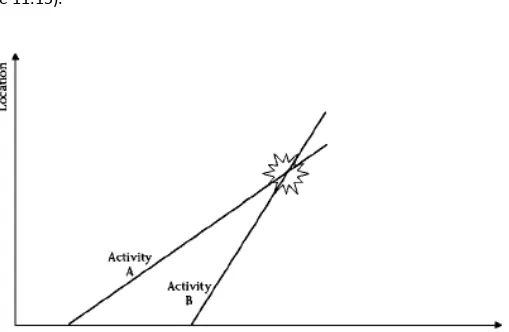
• When we have two or more activities, the production rate will differ from one to another.
• The horizontal distance between two lines represents the float of the earlier activity. In the LSM, we call it the time buffer. The vertical distance represents the distance separating the two operations. We call it the
distance buffer. See Figure below
Buffer: When const. activities progress
example
• a carpentry crew installing and taping drywall for a total of 10,000 square feet (SF).
• The production rate for the crew is 500 SF per day for installation and taping.
• The painting crew is directly behind at a production rate of 800 SF per day.
• Assume that the painting crew starts on day 2 (1 day after the carpentry crew started).
– Then, at the end of day 3, the carpentry crew would have finished 500 x3 = 1,500 SF,
– but the painting crew would have finished 800 x2 = 1,600 SF
There are four solutions for this problem:
1. Speed up the rate of the carpentry crew
2. Slow the rate of the painting crew
3. Make the painting crew start later (calculate the
time buffer)
4. Make the painting crew work in intervals: once
they catch up with the carpentry team, they
• Solution 1 would increase the slope of activity A. (Speed up the rate of the carpentry crew)
• Solution 2 would decrease the slope of activity B. (Slow the rate of the painting crew)
• Solution 3 would increase the time buffer. All three solutions aim at preventing the intersection of the two lines.
• Solution 4 would be represented in an LSM diagram as shown in Figure 11.16. (Make the painting crew work in intervals: once they catch up with the carpentry team, they stop for a period, resume, and so on)
Therefore, alternatively, instead of completely halting activity B during intervals, we can reduce the crew size to slow the rate until there is a safe time buffer (a
• To calculate the time buffer (Figure 11.19), we START FROM THE END: Allow activities A and B to finish simultaneously.
• Then, Duration A = Duration B + Time buffer
Example 11.4
A project consists of five activities:
A. Excavating a trench
B. Laying a sub-base of gravel
C. Laying a concrete pipe
D. Backfilling
E. Compacting
Assume that the length of the pipe is 1,000 LF and that the productivity
rates for the five activities are 100, 125, 75, 200, and 150 LF per day,
respectively. Draw the project diagram, using the LSM. Leave a
Solution
• First, determine the durations by dividing the total quantity, 1,000 LF, by the
production rate for each activity. The following durations result: 10, 8, 14, 5, and 7 days for activities A through E.
• If we start activity A on (end of) day 0, it will finish on day 10.
• Activity B lasts only 8 days and we must leave at least a 1-day time buffer so that we can finish this activity on day 11. Subtracting its duration of 8 days, we find the starting point: day 3.
• Activity C lasts 14 days, so we lag it by 1 day and start it on day 4. It will finish on day 18.
• Activity D can finish no earlier than day 19. It will start on day 14.