REAL TIME DATA MANAGEMENT FOR ESTIMATING PROBABILITIES OF
INCIDENTS AND NEAR MISSES
P.D. Stanitsas a and Y.J. Stephanedes b *
a Graduate Student, Dept. of Civil Engineering, University of Patras, Rio, Greece – [email protected] b Professor, Dept. of Civil Engineering, University of Patras, Rio, Greece – [email protected]
Commission VI, WG 8
KEY WORDS: Real-time, Pattern, Sensor, Vision, Data, Detection, Prediction, Estimation
ABSTRACT:
Advances in real-time data collection, data storage and computational systems have led to development of algorithms for transport administrators and engineers that improve traffic safety and reduce cost of road operations. Despite these advances, problems in effectively integrating real-time data acquisition, processing, modelling and road-use strategies at complex intersections and motorways remain. These are related to increasing system performance in identification, analysis, detection and prediction of traffic state in real time. This research develops dynamic models to estimate the probability of road incidents, such as crashes and conflicts, and incident-prone conditions based on real-time data. The models support integration of anticipatory information and fee-based road use strategies in traveller information and management. Development includes macroscopic/microscopic probabilistic models, neural networks, and vector autoregressions tested via machine vision at EU and US sites.1
* Corresponding Author
1. INTRODUCTION
Transportation and traffic safety has been identified by academics, local authorities and professionals as a critical problem in urban and regional environments. Substantial work has focused in prediction, detection and response to road incidents. However, a generic problem lies in the rarity of these events. Sensors need to monitor large networks around the clock to collect and manage data to be filtered for reduction to potentially useful data sets. Addressing this need, researchers have defined a modelling framework in which crashes and conflicts appear as subsets of a population of events. They then derive relationships between the two subsets, focusing on identifying conditions where data on non-crash events carry information about crashes (Davis, 2003).
Our dynamic models estimate the probability of occurrence of road incidents, such as crashes and conflicts, and incident-prone traffic conditions based on real time data. The models estimate the effect of an additional driver entering the road, on the probability that (a) a capacity-reducing incident or (b) incident-prone traffic conditions will occur. Estimation is based on road geometrics, and dynamic environmental and traffic characteristics. The models are based on results from our research at the EU, NSF, and USDOT, and detailed dynamic data available from EU and US localities.
2. BACKGROUND
Advances in real-time data collection systems, data storage, and computational systems have led to algorithms and integrated systems that can be applied in transportation administration and traffic engineering to improve traffic safety and reduce internal and external cost of transport and traffic operations (Maibach et al, 2008; McDonald and Stephanedes, 2002). Certain problems
in the effective integration of real-time data acquisition, data processing, dynamic modelling, and road use strategies still remain. These are related to increasing system performance in the identification, analysis, detection and prediction of the traffic state in real time (Abdel-Aty and Keller, 2005; Stephanedes, 2004; Banks, 2003).
This research develops dynamic models, including macroscopic and microscopic probabilistic models, neural networks, and vector autoregressive patterns tested by simulation and real data. It supports methods for integrating anticipatory real-time, information and fee-based road use strategies in traveler information and management (Stephanedes et al, 2009). Our macroscopic models are classical high-order models based on continuum mechanics and finite element analysis. Microscopic models are based on theories of driver behaviour, human factors and cellular automata and take advantage of the evolution in computational mechanisms that make the high computational effort in microscopic models achievable.
A substantial portion of the data, especially in microscopic models, is from video recordings. These include raw data collected through surveillance and sensor networks, on specific parts of urban roads and motorways, where unusual traffic conditions are likely to occur. Programmes are developed to filter the raw data through machine vision, and protect and deliver the enhanced data to our models. During this process a number of problems have been identified. Our models are further assisted by data mining processes that support the search for appropriate data patterns prior to application of pattern recognition, vector autoregression or neural networks. Additional data sets are acquired and filtered for evaluating results through machine vision.
3. DATA ENVIRONMENT
Using machine-vision hardware we collect data on several aspects of traffic flow, including traffic state, vehicle speed, vehicle length, average flow rate, traffic volume, arithmetic mean speed, vehicle class, vehicle count per class, average time headway, average time occupancy, level of service, space mean speed, space occupancy, density, stopped vehicle alarm. For a typical motorway section we examine 3-4 lanes for each camera. We place 4 detectors on each lane, two at the beginning and two at the end of the camera frame, detecting presence and speed.
3.1 Data Collection
This section of Data Management contains several difficulties deriving from the individual needs of each type of surveillance network; these vary between microscopic and macroscopic models. In macroscopic analysis a common type of processing is through machine vision software. Once a road scene is defined, multiple cameras are installed such that the total input from their images fulfils detection requirements, and appropriate windows are placed on the road scene such that image artefacts and resulting errors are minimized. Effects from artefacts include, e.g., effects from shadows, sun glare, angle of vehicle movement, distance between vehicles, and unusual vehicle size. Any of the effects can substantially increase identification error.
Addressing this problem, the visual input to machine-vision based systems is transformed, so that higher-level image analysis is facilitated, leading to increased efficiency and cost-effectiveness. Two transformations and methods have been developed, homography-based transformation and panoramic
image reprojection (Tzamali et al, 2006; Zelnik-Manor and
Irani, 2002; Lourakis et al, 2002). Supported by these methods, the data are collected, processed, filtered and stored for algorithm execution in real-time.
Microscopic analysis requires higher data detail in focusing on the interactions between vehicles in a platoon (Davis and Swenson, 2006; Chandler et al, 2005; Davis, 2003). High resolution of video capture is very important to get quality results, and selection of location for camera placement involves many trial receptions before installing the permanent network. Trial receptions could be extracted with portable trailers on locations of potential interest. Considering the high cost of a permanent surveillance network, there is a need for low-error, high-performance design of deterministic or stochastic data networks. Portable trailers play an important role in the design process, offering a cost-efficient solution to data network location design. In addition the trailers can be used for recording periodic phenomena if there is no need for installing a permanent surveillance network. Alternative data collection methods such as GPS and floating car applications, despite measurement error, promise to provide increased efficiency in data management.
3.2 Data Filtering
We use signal filtering to eliminate unwanted frequencies from the received traffic signal. While the correct filter settings can significantly improve signal quality, incorrect settings can severely distort the signal. In what follows, traffic signal filters we commonly use are briefly described.
3.2.1 Exponential Filtering: The exponential filter (equation 1) is the simplest linear recursive filter:
( ) ( ) ( )
t = 1-a *y t-1 +α*x( )
ty (1)
where y(t) is the output of the filter at time t, y(t-1) is the output of the filter at time (t-1), x(t) is the input of the filter,
a is the filter parameter (0≤ a≤1).
3.2.2 Moving Window Filtering: The moving window
(average) filter is most common in traffic signal processing. In spite of its simplicity, this filter is excellent for reducing random noise while retaining a sharp step response. Nevertheless, it is not capable of processing frequency domain encoded signals, because of its reduced ability to separate bands of frequencies. Relatives of the moving average filter include Gaussian, Blackman and multiple pass moving average. The moving average filter operates by averaging data from the input signal to produce output signal and, consequently, introduces an intrinsic time delay in the detection/prediction process. The filter is presented in equation 2:
( )
∑
−[ ]
=
+
1
0
j
i
x
*
M
1
=
i
y
M
j
(2)
where x is the input signal, y is the output signal,
M is the number of points in computing the average.
3.2.2 High Pass/ Band Pass/ Low Pass Filters: The High
Pass filter allows high frequencies to pass, and filters out the low frequencies thus filtering out changes in the signal that occur over a significant period of time. The Band Pass filter only allows the desired band of frequencies to pass, and filters out all others. The Low Pass filter allows low frequencies to pass and filters out the high frequencies, i.e., all portions of the signal that change rapidly, such as electronic noise. A filter commonly used in traffic signal analysis is the low pass Butterworth filter. This filter was implemented on the datasets including vehicle trajectories from a short section of I-680 freeway in California (Hourdos, 2005). Equations 3-5 describe the relationship between input and output in this example.
( )
k =0.4320x(
k-1)
0.3474x(
k-1)
0.1210vin( )
kx1 1 − 2 + (3)
( )
k =0.3474x( )
k-1 0.9157x( )
k-1 0.0294vin( )
kx2 1 − 2 + (4)
( )
k =0.4984x( )
k 2.7482x( )
k 0.0421vin( )
kvout 1 − 2 + (5)
where x1, x2 are the filter state variables,
vin is the input speed signal,
vout is the output filtered speed
3.3 Data Processing
microscopic analysis, this pre-processing step uses macroscopic variables to define useful data. Macroscopic traffic variables are often extracted through machine vision. A strategy for filtering video data is through use of the Fundamental Traffic Diagram (FTD). Most accidents in our data sets occur just prior to the extremum in the FTD.
The algorithm we propose supports reduction of space requirements for data storing. It seeks to achieve such reduction through differentiating amongst data by flow state in the FTD. Using the state of flow, data are classified into free-flow, transition-flow or saturated-flow.
3.4 Data Storage
Owing to space limitations data storage is a demanding part of Data Management. Storing data later found to be of little relevance decreases available space and limits the amount of relevant data that are stored. Storage challenges depend on the type of analysis. In macroscopic analysis, using machine vision software, we collect data from all detectors at time interval of 1 millisecond. The space required is proportional to the number of detectors placed on each camera, and the number of cameras. In a simple example that follows, a description of the typical space required per second is presented.
After the results deriving from the algorithm are harvested and categorized we define the data with storing value. In this research the data corresponding to the High Risk part of the fundamental diagram were stored. Finally these datasets are stored in external hard drives, and each drive is labeled according to its content.
4. ALGORITHM DEVELOPMENT
The algorithm proposed in this paper is developed to estimate, in real time, future probabilities of incidents, near-incidents and incident-prone conditions based on the flow state, while maintaining efficient data storage. The basic measurements to distinguish the data through machine vision are q (traffic volume) and k (traffic density). Each point of the FTD is represented on a q-k coordinate system. Most incidents tend to occur at the part of the fundamental diagram that describes the transition from free flow to saturated flow. In our work the part describing that transition will be called “High-Risk” part.
Initially the algorithm goes through a learning process to define the bounds of High-Risk in the FTD. Using an incident detection process, information regarding actual incidents is collected and stored. According to previous work in freeway incident detection through filtering (Stephanedes and Chassiakos, 1993) the measurements used to determine the existence of an incident are smoothed values for occupancy at two consequent time periods gathered from two stations. Two tests are performed.
The first test, described in expression 6 examines current spatial occupancy difference to detect congestion between stations i and i+1. The difference is normalized by the difference in occupancy between the two stations during the past period to reflect changes relative to previous traffic conditions, and compared to congestion test threshold, T1.
{
}
1 incident test threshold, T2.[
] [
]
given the incidents, are calculated and the bounds of the High-Risk partition are determined.The second part of the algorithm is responsible for separating the values gathered through machine vision. A comparison between High-Risk bounds and (qi, ki) pair is made at every ith second. Depending on the result of this comparison an updated partition label is placed on every set of values. This labelling process supports the selection of subspaces in which to form future patterns. Depending on pattern recognition objective, we modify the emphasis on the types of clustering on which the patterns are based. The label placed on each set of values includes the flow state of the N-1 previous values, where N is the number of consecutive values that are grouped and stored together; N is user-defined. Inclusion of this historical element differentiates amongst data orbits allowing, e.g., transition data that migrate from free flow to saturated flow to have different meaning from data deriving from free flow only.
At the final part of the algorithm a pre-storing process takes part. In this stage values are grouped and stored in sets of N. Entropy for each set is calculated and stored together with the set. The natural definition of entropy (also referred to as sample
entropy) in this setting is defined in Equation 8.
∑
extraction is used. Given the increasing size of traffic data in real time, the method supports estimation of predictive patterns by efficient pre-selection of the most relevant data. Such methods are, e.g. Karhunen-Loeve (Watanabe, 1967); minimax entropy (Christensen, 1981). With minimax entropy, this is achieved in two steps, (a) the conditional outcome global entropy defined for the desired events is minimised with respect to characteristics of class boundaries such as q and k, and updates the relevant FTD class boundaries for which this entropy is minimum; (b) entropy maximisation supports assignment of value to each event probability by maximising the unconditional local entropy of the subset of events while minimising bias.
In applying minimax entropy, data storage is a key element for two reasons. First, the maximum entropy probabilities for the defined class events approach data frequencies in the limit of large sample sizes. Second, event classification via entropy minimisation is relative to the data on past events. With a large number of real-time traffic variables upon which event estimation may depend, where the interrelations amongst these variables may be insufficiently understood or are too complex, the required data storage can be large. This requirement could still be preferable when compared to other alternatives such as exhaustive use of sample averages. For example, under Poisson statistics, holding uncertainty I in an outcome probability of events down to I = (N)-1/2, for all possible range combinations, by exhaustive use of sample average estimates, requires sample size N = GK I-2 with K the number of independent variables, G the number of significant ranges of value for each, and events evenly distributed over these ranges; for large G, K, attaining the required sample size might not be realistic.
Storage efficiency can be improved through Kalman filtering in the learning process. Kalman filtering allows the boundaries of High Risk partition of the fundamental diagram to respond to changes in entropy. Entropy can be calculated a priori for the 3 different traffic states, and then be calculated anew when a certain number of new pairs of (q,k) are added to each category. Implementing the Kalman filter can be activated by two tests, described in expressions 9 and 10.
∑
(
x
i+
k
i)
*
ln(
x
i+
k
i)
≺
∑
x
i*
ln(
x
i)
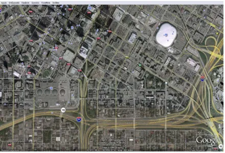
(9)The proposed algorithm was implemented on processed video datasets from two motorway sections, (a) 2.7-km, 3-lane urban section of interstate I-94 in Minneapolis, Minnesota (Fig. 1) and
(b) 5.4-km, 4-lane urban section of national road E-75 in Athens, Greece (Fig. 2).
Figure 1. I-94 freeway, Minnesota
The section of I-94 includes 2 entrance ramps and 3 exit ramps. It exhibits traffic volume of 80,000 vehicles each way, traffic congestion for 5 hours daily and 4.8 crashes/M veh-mile, practically one every other day. This site provides a large number of rear end collisions and other unusual traffic phenomena. Major cause is the geometry, i.e., an exit ramp shortly after an entrance ramp, and an unlawful early merging at the following entrance ramp. This geometric-demand environment produces severe shockwaves on the right lane.
Figure 2. E-75 motorway, Athens
The E-75 section includes 3 entrance ramps and 3 exit ramps, and exhibits severe congestion during 7 hours daily. The road geometrics include closely spaced exit and entrance ramps, and a two-lane reduction at a horizontal curve prior to a high-demand exit/ entrance ramp combination. This geometric-demand environment produces several traffic phenomena daily, including several shock waves.
the High Risk partition of the fundamental diagram. Our datasets are stored in a storage array of hard drives placed on DroboPro hardware, and this allows total storing space of approximately 16 terrabytes. Each time a hard drive reaches its capacity, it is labeled and stored, and a new, empty drive is placed in DroboPro.
Experimental setup is similar at each of the two research sites, I-94 and E-75 sections. At each section, we place 4 detectors per lane per camera, two at the beginning and two at the end of camera frame, detecting vehicle presence and vehicle speed, for a total of 12 detectors per frame. At both sites, presence detectors are updated every second saving values for all traffic variables at the output, and speed detectors are activated at the time (millisecond) that a vehicle crosses and activates the detection point, for a total update of at least 15 variables every second for each detector. If three characters are saved, for every variable derived from presence detectors we store 2 Kb per second on average. To this requirement, we add 1 kb deriving from speed detectors and 400 bytes for file information and information regarding time characteristics, totalling 3.4 kb per second for each camera. The network harvests information for 8 hours per day leading to 100 Mb of storage space required per day, per camera. On the 2.7-km I-94 section, 4 cameras are operating and this produces the need for 400 Mb storage per day. On the 5.4-km E-75 section, with 6 cameras operating the need per day is increased to 600 Mb.
In microscopic analysis we focus on the details of the interactions amongst interacting vehicles, primarily during a shock wave, that end with a near miss or rear end collision. Time interval is usually 0.1 second. For each time interval, a pair of Cartesian coordinates referring to the trajectory of each vehicle in a platoon is saved. Considering that an average near miss includes a 240-s trajectory, and a typical platoon may consist of 6 vehicles, 4 Mb are needed for each platoon in a near miss. With approximately 1-5 platoons involved per near miss, 4-20 Mb per near miss are required. Several (e.g., 10-20) near misses are produced daily resulting in a data storage need of up to 400 Mb per day.
In addition we consider, especially in microscopic analysis, the video data that are bonded with the graphs and trajectories of each near miss and need to be stored as well. The calculation for microscopic analysis is applicable to off-line analysis of stored data, in which the near misses have already been identified. Real-time data requirements equivalent to macroscopic analysis collection procedures would lead to 2.4 Gb per 8-hr weekday for the locations of interest in the 2.7-km I-94 section. Owing to increased resolution requirements, installation of additional cameras is required leading to increases in storage needs. Estimated required storage space for microscopic and macroscopic analysis at this site is summarised in Table 1.
______________________________________________ Type of Analysis Daily storage requirements __________________________________________________ Macroscopic 400 Megabytes
Microscopic 2.4 Gigabytes
Total 2.8 Gigabytes
__________________________________________________
Table 1. Storage space requirements at I-94 section
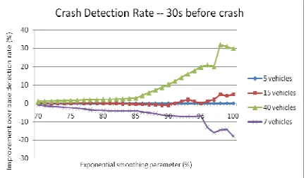
Algorithm performance in detection of incidents and near-incidents varies with type of pre-processing and filtering. A typical performance curve indicating range of performance for filtering parameter ranges in I-94 is presented in Figure 3. From the figure, moving averages of larger numbers of vehicles improve Detection Rate of a crash for the range of exponential smoothing parameter, 30 s before the crash. Dynamic analysis of performance measures can support real-time selection and updating of values for data filtering but requires additional storage.
Figure 3. At 30s before crash, Detection Rate is compared across values of moving average of vehicles (base case=5veh)
6. SUMMARY
This research develops dynamic methods for incident prediction, including macroscopic and microscopic probabilistic models, neural networks, and vector autoregressive patterns that are tested by simulation and real data. The methods support integration of anticipatory real-time, information and fee-based road-use strategies in traveller information and management systems. Raw data are collected through road surveillance systems and sensor networks, and filtered through machine vision.
An algorithm is developed for estimating, in real time, future probabilities of incidents, near-incidents and incident-prone conditions based on the flow state, while maintaining efficient data storage. The algorithm is based on traffic volume and traffic density, and other variables derived from these. It is supported by the fact that most incidents tend to occur at the transition of the fundamental diagram from free flow to saturated flow, a transition we call High-Risk. A learning process defines the bounds of the High-Risk partition using an incident detection process, information on actual incidents, and two tests against congestion and incident thresholds. An update of the High-Risk partition and every set of new data is made at every second.
using minimax entropy. Storage efficiency can be improved through Kalman filtering.
Algorithm performance in the detection of incidents and near-incidents is tested at two urban motorway sites in I-94, Minneapolis, Minnesota; and E-75, Athens, Greece. Performance varies with type of pre-processing and filtering. For example, at I-94 moving averages of larger numbers of vehicles improve Detection Rate of a crash for the range of exponential smoothing parameter, 30 s before the crash. Real-time data requirements for macroscopic and microscopic analysis at the 2.7-km, 3-lane I-94 site lead to 2.4 Gb per 8-hr weekday. Dynamic analysis of performance measures can support improved real-time selection and updating of values for data filtering but requires additional storage.
REFERENCES
Abdel-Aty, M. and Keller, J., 2005. Exploring the overall and specific crash severity levels at signalized intersections,
Accident Analysis and Prevention, 32, pp. 633-642.
Banks, J.H., 2003. Average Time Gaps in Congested Freeway Flow, Transportation Research Part A: Policy and Practice, July, 37(6), pp. 539-554.
Chandler, R.E., Herman, R., and Montroll, E.W., 2005. Traffic Dynamics: Studies in Car Following, Operations Research, 6(2), pp. 165-184, March - April.
Christensen, R., 1981. Entropy Minimax Sourceboook, Entropy Ltd., Lincoln, Massachusetts.
Davis, G.A., 2003. Bayesian Reconstruction of Traffic
Accidents, Law, Probability and Risk, 2(2), pp. 69-89.
Davis, G.A. and Swenson, Tait, 2006. Collective Responsibilty
for Freeway Rear-Ending Accident? An Application of
Probabilistic Causal Models, Accident Analysis and
Prevention, July, 38(4), pp. 728-736.
Hourdos, J., 2005. Crash Prone Traffic Flow Dynamics:
Identification and Real Time Detection, PhD. Dissertation,
Department of Civil Engineering, University of Minnesota, Minneapolis, USA.
Lourakis, M.I.A., Argyros, A.A., and Orphanoudakis, S.C., 2002. “Plane detection in an uncalibrated image pair.” Proc.,
British Machine Vision Conference, British Machine Vision
Association, Worcs, UK, 2: 587-596.
Maibach, M., Van Essen, H.P., Boon, B.H., Smokers, R., Schroten, A., Doll, C., Pawlowska, B., 2008. Handbook on
estimation of external costs in the transport sector, version 1.1,
CE, Delft.
McDonald, M., and Stephanedes, Y. J., eds., 2002. Prediction
of congestion and incidents in real time, for intelligent incident management and emergency traffic management, Fin. Report,
PRIME IST-13036, Brussels, Belgium.
Stephanedes, Y.J., Davis, G.A. and Hourdos, J., 2009. “Dynamic freeway management based on real-time estimation of incidents and incident-prone traffic conditions,” Proc.,
Second International Symposium in Freeway Operations, 21-24
June, Transportation Research Board, Hawaii.
Stephanedes, Y. J., 2004. “Intelligent Transportation Systems.”
The Engineering Handbook, 2nd Ed., R. C. Dorf, ed., CRC
Press, Boca Raton, Florida, Ch. 86, ISBN 0-8493-1586-7.
Stephanedes, Y. J., and Chassiakos, A., 1993. “Freeway incident detection through filtering.” Transportation Research
Journal, 1C(2), pp. 219-234.
Tzamali, E., Akoumianakis, G., Argyros, A. and Stephanedes, Y.J., 2006. Improved Design for Vision-based Incident Detection in Transportation Systems Using Real-Time View Transformations. ASCE J. of Transportation Engineering, 132(11), pp. 837-844, Manuscript no.: TE/2005/023349, November.
Watanabe, S., 1967. “Karhunen-Loeve expansion and factor analysis, theoretical remarks and applications,” Trans. of the
Fourth Prague Conf. on Information Theory, Statistical Decision Functions, Random Processes, Prague, Aug. 31-Sept.
11, 1965, Academia, Publ. House of the Czechoslovak Academy of Sciences, Prague, pp. 635-660.
Zelnik-Manor, L., and Irani, M., 2002. “Multiview constraints on homographies.” IEEE Transactions on Pattern Analysis and
Machine Intelligence, IEEE, N. York, NY, 24(2), pp. 214–223.
ACKNOWLEDGEMENTS
This work was partially supported by the European Union. We acknowledge the U.S. Braun Intertec Committee for supporting the basic research, “Models of Congestion and Incident Prediction,” that has provided the seed for this work. We thank Dr. J. Hourdos, Director of Minnesota Traffic Observatory, for making available most data, Dr. G. Davis for his assistance, and the Departments of Civil Engineering of the University of Minnesota and of the University of Patras for supporting this international cooperation.