*Corresponding author
MODELLING OF AN INEXPENSIVE 9M SATELLITE DISH FROM 3D POINT CLOUDS
CAPTURED BY TERRESTRIAL LASER SCANNERS
D. Belton1,2*, A. Gibson2, B. Stansby3, Steven Tingay3 and K.-H. Bae2 1
Cooperative Research Centre for Spatial information (CRC-SI),
2 Department of Spatial Sciences, Curtin University of Technology, Perth, WA, Australia 3 Curtin Institute of Radio Astronomy, Curtin University of Technology, Perth, WA, Australia
Commission V, WG V/3
KEY WORDS: Terrestrial Laser Scanners, 3D point clouds, Modelling, Classification
ABSTRACT:
This paper presents the use of Terrestrial laser scanners (TLS) to model the surface of satellite dish. In this case, the dish was an inexpensive 9m parabolic satellite dish with a mesh surface, and was to be utilised in radio astronomy. The aim of the modelling process was to determine the deviation of the surface away from its true parabolic shape, in order to estimate the surface efficiency with respect to its principal receiving frequency. The main mathematical problems were the optimal and unbiased estimation the orientation of the dish and the fitting of a parabola to the local orientation or coordinate system, which were done by both orthogonal and algebraic minimization using the least-squares method. Due to the mesh structure of the dish, a classification method was also applied to filter out erroneous points being influenced by the supporting structure behind the dish. Finally, a comparison is performed between the ideal parabolic shape, and the data collected from three different temporal intervals.
1. INTRODUCTION
Terrestrial laser scanners (TLS) have seen many applications in modelling and monitoring surface structures and their deformations (Gordon et al., 2003). As technology develops, this increasingly includes high precision applications and, for example, large satellite dishes for radio astronomy were successfully measured and modelled by TLS (Sarti et al., 2009). This paper presents such an application of TLS to determine the surface model of an inexpensive 9m dish in order to gauge its quality and efficiency. This formed part of a project to investigate the use of low cost dishes for statistical survey work (where orientating the dish was not a primary factor) against traditional dish systems that were of a significant cost. The processing of the data is performed in several stages. After capturing of the data is complete the orientation of the dish is approximated and an initial parabola is fitted. An outlier detection and classification method is applied to identify and remove outliers and extraneous data. The surface is then modelled and the root mean square (RMS) value is calculated to approximate surface efficiency. Capture was performed for three different epochs to test repeatability and the ability to detect change in the surface.
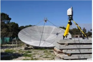
Figure 1: Satellite dish and the setup of the scanner to capture the surface.
2. BACKGROUND
The surface of a dish conforms to a parabolic shape so that the signals reflected of the surface are focused at the receiver. The maximum gain of the signal and the receiving frequency range is determined by primarily by the diameter and surface of the dish. However, imperfections in the surface will result the reduction of its signal reception and a smaller range of observable wavelength for the dish. These imperfections can be caused by construction, surface undulations, changes in orientation and deformation over time, and is present in all dishes to some extent. Typically, a dish that has a surface efficiency of 65-70% for a particular wavelength is considered to be optimal (Thompson et. al., 2001).
The amount of surface efficient for a dish can be formulated as a function of the error in the dishes surface, which is well known as Ruze’s equation (Ruze, 1966), as follows:
(1)
where L is the percentage of signal reception efficiency, G and G0 are the observed gain and the maximum gain for a perfect surface, respectively, λ is the wavelength and ε is the effective
reflector tolerance. In this case, ε is taken as the RMS of the surface to a true parabola.
To measure the surface error, photogrammetry and holography have effectively been used either to obtain accurate surface measurements, or to compare it to the signal of another receiving dish (Bolli et al., 2006). Photogrammetry needs to use large numbers of reflective targets in order to ensure its high metric precision, which may not be possible in certain cases. Holographic methods can be applied without the targets but precision mapping and identification of surface imperfections are not possible (Thompson et. al., 2001). Furthermore, the
spatial coverage of photogrammetric methods can be narrow since it is totally dependent on its target setup on the dish. Alternatively to these methods, TLS can be utilised to capture data points for modelling surfaces. Such a procedure has been applied to VLBI (Very Long Baseline Interferometry) telescopes as described in Sarti et al. (2009).
TLS has been previously employed in a variety of applications to model objects and surfaces with high accuracy (Schulz, 2004). The point accuracy of the sampled points from TLS may be greater than those achieved using traditional photogrammetric and surveying techniques depending on the individual instrument, but benefits are gained from the fast acquisition of high volumes of 3D point data (Jansa et. al., 2004). The advantage of dense sampling is it allows detection of small imperfections in the surface, which may not be recognisable with a sparser data set. Much accurate modelling is also possible due to its high spatial density with possible systematic errors from the TLS, which can only be removed by a calibration procedure. Furthermore, since the raw points are originally captured in 3D, there is no post-processing of the data as required by traditionally photogrammetry. Finally, the data is able to be captured without direct contact to the surface without reflective targets.
3. TEST SITE
The focus of this paper was an inexpensive satellite dish, 9 metres in diameter, with a focal length of approximately 3.42m, and was manually constructed for radio astronomy. Surface data was captured using a Leica ScanStation (Leica, 2011), with a range error of approximately 2mm. Figure 1 depicts the dish modelled and the scanner setup relative to the orientation of the dish. There were several factors involved in the capture of the data. The first was that the dish had a limited ability to change its orientation. Unlike the method presented in (Sarti et. al., 2009), there was no ability to access or mount the scanner in the centre of the dish. This meant that the dish had to be orientated to the side and the scanner situated on top of a raised platform. Care had to be taken to ensure the stability of the platform, and the absence of environmental factors such as wind, which would affect the accuracy of the captured data.
Because of the limited viewing angle, there was the presence of high incident angles to the dish from the TLS, as illustrated in Figure 1. While this does not impact on the location of the sampled points, it does mean that the effect of the point uncertainty is not homogeneous over the entire surface (Bae et al., 2009).
The last experimental consideration was the construction of the surface. For this dish, the surface was formed out of mesh panels. This may cause two effects in the surface data. The first is that the surface is textured and not smooth as if solid panels were used, which may result a higher RMS value to the orthogonal direction to the local surface. The second effect is that the laser beam will pass through the mesh to sample the underlying surface, which causes the sampled point being biased due to the return signal comprising of a mix the dish surface, and the underlying support structure. As highlighted in Figure 6, this effect can even visually observed, when laser beams’ incidence angle is nominally aligned to the angle of the holes in the mesh. To remove these erroneous points, a classification technique was applied to the raw point clouds, which will be describe in the latter section.
4. MODELLING THE DATA
4.1 Parabolic surface fit
The ideal parabolic surface was fitted to the point cloud using least squares. The formulation of the problem was considered in two parts; finding the orientation of the dish with respect to the scanner orientation, and then fitting a parabola to the points sampled to the dished surface in the local orientation of the dish. 4.1.1 Orientation
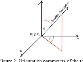
As presented in Figure 2, we introduce a coordinate system where its origin is located at the minimum of the parabola and the z-axis is aligned to the centre axis of the dish. The x-axis is constrained as being perpendicular to the z-axis to restrict rotation around the centre axis. To solve for the transformed coordinate system, three translation parameters and two rotation parameters are required. The three translation parameters (x0, y0, z0) represent the location of the origin at the bottom centre of the dish. The two rotation parameters are specified as a rotation around the vertical z-axis (φ) and a rotation from the vertical
z-axis (θ). These angles reflect the physical orientation or
alignment of the dish as shown in Figure 2.
Figure 2. Orientation parameters of the test dish. The rotation matrix defining the orientation is defined using the two angles as
(2)
The transformation of points from the scanner orientation into the local orientation of the dish is then specified as
(3) where R is the rotational matrix specified in equation (2), X0 is the origin of the local coordinate system for the parabola and Xi is a point observed in the scanner coordinate system. A method for finding the initial approximate values for this transformation is outlined in section 5.
4.1.2 Parabola formula
Once the sampled points are in the local coordinate system of the dish, the equation for the parabola of the surface is simply
(4)
where x’, y’ and z’ are in the transformed coordinates system defined by equation 2. The value f represents the focal length of the dish, and defines the nominal position of the receiver as (0,0,f), with respect to the local coordinate system of the dish. This is from the fact that signals propagating parallel to the direction of the z’ axis will reflect off any given point on the dishes surface defined by (4), and intersect at this point.
4.1.3 Combining two parts
In order to obtain the functional model F or the condition equation for the problem, Equations 3-4 can be combined as follows:
This can then be linearised in the form of
with partial derivatives of F with respect to the parameters, and r denoting the residual. Formulation of the least squares problem in matrix form is given as
(7)
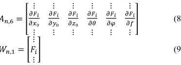
where δ contains the optimal correction for the parameters x0, y0, z0, θ, φ and f, and A and W are the design and misclosure matrix defined, respectively, as
(8)
(9)
The points captured from the laser scanner can be used to solve the parameters and find the residuals from the surface fit. 4.2 Algebraic fitting and geometric residuals
It should be noted that the least square fit of the parabola is based on the algebraic distance of the points to the surface. In this case, this means that the residuals calculated are based on the distance of the sampled points to the fitted surface in the z’-axis direction of the local dish coordinate system. As illustrated in Figure 3, these algebraic residuals r(z) from the least squares solution will be significantly different from the true orthogonal residuals r, which is based on the distance of point to the surface in the surface normal direction. To determine the true RMS of parabola, these residuals must be corrected.
4.2.1 Ortho-normal Least Squares fitting
While it is possible to derive the functional model in terms of the orthogonal distances between the points and the surface (Ahn et. al., 2001), it was not applied in this case. The reason was that while fitting the algebraic surface may introduce some biasing, in this case there will be no observable difference to the geometric surface formulated using orthogonal residuals. This is due to the parabolic surface being relatively shallow and being fitted to the local orientation as depicted in Figure 2. For this reason, the algebraic surface is fitted and the residuals are corrected to reflect the orthogonal distances.
Figure 3: The algebraic residual compared with the orthogonal residual for a point.
4.2.2 Exact Solution
In figure 3, the relation between the sampled point (xi, yi, zi) to the closest point on the surface (x, y, z) is sketched in 2D. For the local coordinate system of the dish at point (x, y, z), the normal direction can be approximated for partial derivatives as
(10)
The position of the sampled point can then be given in relation to the closest point based on the parametric function defined as
(11)
Equation 11 represents that the difference between the sampled point and the closest point on the dishes surface will be defined by some multiple s of the vector representing the normal direction defined in equation 10. This system can be solved to find the x, y values of the closest orthogonal point on the dish, and the s to determine the distance in terms of the multiples of the normal direction
4.2.3 Approximate Solution
For the previous method solving equation 11, it is not trivial to obtain the closed form solution, as it requires factorisation of a third order polynomial. Instead a simple method to approximate the solution is proposed, which locally projects the residual r(z) onto the surface normal at (xi, yi), as illustrated in Figure 3. The unit normal direction is specified as
(12)
And the projected residual r(z) onto the normal direction gives an orthogonal distance of
(13)
As can be seen in Figure 3, it is not the exact solution and will still slightly overestimate the residual. For a focal length of f=3.42 at a radial distance of 4m from the origin with a value of r(z)=0.006, the approximate value was calculated as r(a)=0.0051794m, compared to the true value of r=0.0051789m.
In this case, the difference between r and r(a) is insignificant, but the difference between r(z) and r(a) is significant, especially towards the edge of the dish. For example, Figure 4 shows the differences between r(z) and r(a) as a percentage with respect to the radial distance of the point to the centre of the dish. This shows a potential difference of up to 16.46% between residual values at the edge of the dish.
Figure 4: The difference between the algebraic residuals and the approximated orthogonal residuals. The x axis is the radial distance of the point to the centre of the dish and the y axis is
the percentage difference between r(z) and r(a).
Figure 5: Residual map of the fitted dish using algebraic residuals with a RMS of 0.0031m. The axes represent the local
x and y coordinate system of the dish, with the bottom of the dish (closest to the ground) towards the right of the figure.
Figure 6: Residual map of the fitted dish using orthogonal residuals with a RMS of 0.0028m
Figure 5 presents the algebraic residual plot while figure 6 presents the corrected residuals over the dishes surface from the parabola fit outlined in Section 4.1.3. A slight reduction in the residuals, especially towards the edge of the dish, can be seen between the respective figures and a reduction in the RMS of the surface fit from 0.0031m to 0.0028m is observed.
4.3 Cleaning and refining the data
The majority of the data cleaning was performed using Cyclone (Leica, 2011), the software used to capture the raw data. This was done by firstly removing the extraneous points around the dish, and then fitting a smooth surface to the actually surface of the dish. A loose tolerance was used at this stage that was significantly larger than the point uncertainty to ensure all point on the surface were included, while removing the majority of the sampled points captured from surrounding structures, frame work and the receiver legs. The fitting routine for the parabola was then applied to get the initial orthogonal surface fit and corresponding residuals. An outlier detection procedure was then applied to remove points deemed to not belong to the surface model of the dish.
Because of the mesh material of the dish, points on the supporting structure are also sampled. As previously mentioned, a problem may arise because, due to the beam diameter, some of the return points will be a blend of return signals from supporting structure and the dish surface (Lichti, 2004). This causes points on the mesh surface where the structure can be seen to be skewed slightly behind the dish, as seen in the residual plot in Figure 5.
Because the differences observed between the biased points and the points sampled on the surface are small (order of millimetres), outlier detection will not always eliminate these points. To remove them from the surface modelling, a classification method is utilised to try and identify these points. The method employed is based on the variance of curvature (Belton et al. 2006). The first step is to find the curvature of the surface using local neighbourhoods. The curvature is found using principle component analysis (PCA) on a small local neighbourhood, as outlined in Pauly (2002). Points with high curvature will relate to local regions of high variation in the point surface, such as those cased by the biasing occurring from the supporting structure. Such points can be classified if they exceed a threshold value.
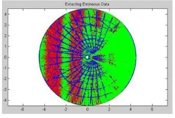
Figure 7: Classification of points. Green and red points denote surface and high curvature points, respectively. Blue denote
discontinuities in local curvature information. The axes represent the local x and y coordinate system of the dish, with the bottom of the dish (closest to the ground) towards the right
of the figure.
For the case of the satellite dish present in this paper, the results are shown as non-green points in figure 7. As can be seen, there are large regions of such classified points. This could be due to a combination of the angle of the hole in the mesh, the incident angle and anomalies in the instrument. To filter out the points that are being biased, the variance of curvature is used as an indicator, which approximates the second order surface change. A low variance of curvature indicates that local surface in the
neighbourhood is consistent. A high variance of curvature indicates the surface undergoes a change and is not consistent. A decision is based on threshold values in the form of
(14)
where the thresholds are adjusted until only the biased points are classified. Such classified points are indicated by blue points in Figure 7.
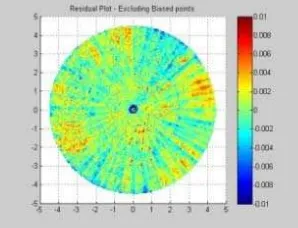
Figure 8: Residual plot of the dish after classified biased points have been removed, with a RMS of 0.0024m.
The classified points represent the majority of the biased points and can be used remove such points from the modelling process. A plot of the modelled residuals is shown in figure 8. With the biased points included a RMS value of 0.0028m was obtained, compared to a RMS value of 0.0024m when the majority of these points have been classified and removed. While this improves the modelled surface, how the physical effect causing the biased point will affect the surface efficiency of the dish is not known.
5. RESULTS
Three separate scans were taken at different dates. The first was before the antenna feed was installed, the second several days after the receiver and legs were in place, and the third was taken just over eight months after the second scan. Initial orientation parameter values were found from a plane fit and the focal length from the manufacturer’s specification. A plane was fitted using PCA to the data points to determine the normal direction and the lowest point with respect to orientation of the dish. The normal direction ([nx, ny, nz]
T
) was used to approximate the orientation of the dish by
(15) (16)
where the lowest point was used to approximate the origin of the point.
An initial parabola fit was performed as specified in Section 4.1. The results were used to test for outliers. To limit the effects of the scanner beam passing through the mesh, the classification process highlighted in Section 4.3 was used to remove and limit the effects of the points biased by the underlying support structure. A parabola was then refitted to the remaining points. The results are presented in Figure 9 in the form of a residual map over the surface of the dish.
The focal lengths values are approximately equivalent for each scan epoch to within 2mm. These focal length values are presented in Table 1, along with the RMS value for each scan.
(a) (b)
(c) (d)
(e) (f)
Figure 9: Residual plot of the dish on (a) 9 Dec 2008, (c) 15 Dec 2008 and (e) 27 August 2009. (b) is the difference between
the 9 Dec 2008 and the 15 Dec 2008. (d) is the difference between the 15 Dec 2008 and the 27 Aug 2009. (f) is the difference between the 9 Dec 2008 and the 27 Aug 2009.
Date RMS Focal Length
9 Dec 2008 0.00237 3.4419
12 Dec 2008 0.00275 3.4400
27 Aug 2009 0.00250 3.4414
Table 1: RMS and focal length values of the parabola fit for the different setup dates.
A jump in the RMS value can be seen between first and second scan. This coincides with the installation of the receiver and support legs. The effect of installing the receiver legs can be seen in Figure 9(b). Looking at the difference in residuals between the first and second scan, a deformation at roughly 120o intervals at the edges of the dish shows the effect of the receiver legs on the shape of the dish. There is no significant observable difference in the residual plot between the second and third scan, as shown in Figure 9(d), except where the biased points from the underlying structure have not entirely been removed, however there is a decrease in the RMS value between the second and the third scanning period. This could indicate the overall deformation caused by installing the antenna legs settling over time, or that the second scanning period was affected by an unknown external. Additional scans need to perform to clarify this.
The observed RMS value will be comprise of two parts, the point uncertainty (σi), and the error caused by surface imperfections of the dish from the true parabolic shape (σs).
(17)
For the Lecia Scanstation used in this paper, the modelling error
(σi) is approximately 0.002m. This means a RMS of over 0.002m will have a noticeable error caused by the surface imperfection. However, if the RMS was less than that, it is difficult to quantify the error caused by the surface not conforming to a parabola, as the effect will be eclipsed by the uncertainty in the modelling. To reduce the effect of point uncertainty, a more precise instrument may be used, such as a phase based close range scanner.
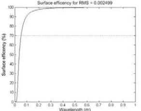
In the case of this paper, the quality of in the construction of the satellite dish, as well as the mesh surface does seem to give rise to a significant RMS value resulting from the deformation of the dishes surface from a parabola. Using laser scanning also highlights observable trends in the dishes surface due to the dense sampling rate. This is demonstrated in the observable patterns in the surface residuals caused by slight differences between the mesh sections. The comparison between the residual surfaces before and after the receiver legs have been installed also demonstrates the ability to detect change between scanning epochs. If the RMS value from Figure 9(a) is utilised to model surface efficiency, the trend in figure 10 is observed. Based on 70% optimal achievable surface efficiency, the minimum wavelength that can be observed at such is approximated at 0.0526m.
Figure 10: The surface efficiency against wavelength for the surface modelled in the last scanning epoch. The vertical axis is
the surface efficiency as a percentage value against the horizontal axis denoting the wavelength in metres,
6. CONCLUSION
This paper has demonstrated the use of TLS point cloud data in modelling the surface of satellite dishes. It illustrates the ability to detect deformations in the dish from the ideal parabolic surface and between successive scans, and how the observed RMS value can be used to predict the surface efficiency. The modelling accuracy of the instrument will determine the minimum effect of surface that can be quantified. In the example presented in this paper, the focus was an inexpensive dish, and the level of accuracy was more than capable of detecting the impact on surface. It also showed how the effects of the support structure being sampled through the mesh surface can be indentified using simple classification techniques. In the future, effects such as temperature, orientation and gravitational forces will need to be taken into consideration.
ACKNOWLEDGEMENTS
This work has been supported by the Cooperative Research Centre for Spatial Information, whose activities were funded by the Australian Commonwealth’s Cooperative Research Centres Programme. Thanks also to the Radio Astronomy Group at Curtin University.
REFERENCES
Ahn, S. J., Rauh, W. and Warnecke, H. –J., 2001, Least-squares orthogonal distances fitting of circle, sphere, ellipse, hyperbola, and parabola. Pattern Recognition 34, pp 2283-2303.
Bae, K.-H, Belton, D. and Lichti, D.D. 2009, A Closed-From Expression of the Positional Uncertainty for 3D Point Clouds. IEEE Transaction on Pattern Analysis and Machine Intelligence 31 (4), 577- 590.
Belton, D. and Lichti, D. D., 2006. Classification and segmentation of terrestrial laser scanner point clouds using local variance information. International Archives of the Photogrammetry, Remote Sensing and Spatial Information Sciences Vol XXXVI, Part 5, pp. 44–49.
Bolli, P., Montaguti, S., Negusini, M., Sarti, P., Vittuari, L. and Deiana, G. L. 2006. Photogrammetry, Laser Scanning, Holography and Terrestrial Surveying of the Noto VLBI Dish. in IVS 2006 General Meeting Proceedings pp. 172-176.
Gordon, S. J., Lichti, D. D. and Stewart, M. P. 2003. Structural deformation measurement using terrestrial laser scanners. In Proceedings of 11th International FIG Symposium on Deformation Measurements. Santorini Island, Greece
Jansa, J., N. Studnicka, Forkert, G., Haring, A., and Kager, H, 2004. Terrestrial laserscanning and photogrammetry - acquisition techniques complementing one another. International Archives of Photogrammetry, Remote Sensing and Spatial Information Sciences VOL. XXXV, Part B5.
Leica Geosystems HDS 2011. [Website]
accessed:
April 2011.
Lichti, D. D. 2004. A Resolution measure for Terrestrial Laser Scanners, The International Archives of the Photogrammetry, Remote Sensing and Spatial Information Sciences, Vol. 34, Part XXX.
Pauly, M., Gross, M. and Kobbelt, L. P. 2002. Efficient simplification of point sampled surfaces. In VIS ’02: Proceedings of the conference on Visualization ’02, Boston, Massachusetts, pp. 163–170. IEEE Computer Society. Ruze, J., 1966. Antenna Tolerance Theory – A Review,
Proceedings of the IEEE, 54(4) pp. 633-640.
Sarti, P., Vittuari, L., and Abbondanza, C. 2009. Laser Scanner and Terrestrial Surveying Applied to Gravitational Deformation Monitoring of Large VLBI Telescopes’ Primary Reflector. Journal of Surveying Engineering 135(4), pp. 136-148.
Schulz, T. and Ingensand, H. 2004. Terrestrial Laser Scanning - Investigations and Applications for High Precision Scanning. In: Proceedings of the FIG Working Week - The Olympic Spirit in Surveying, Athens.
Thompson, A. R., Moran, J. M. and Swenson G. W. 2001. Interferometry and Synthesis in Radio Astronomy (2nd ed.), Wiley-VCH, Germany.