ANALYSIS AND APPLICATION OF LIDAR WAVEFORM DATA USING A
PROGRESSIVE WAVEFORM DECOMPOSITION METHOD
Junfeng Zhu a, Zuxun Zhanga,Xiangyun Hu a, *, Zhen Lia a
School of Remote Sensing and Information Engineering, Wuhan University, Wuhan 430079, China-
[email protected], [email protected], [email protected]
KEY WORDS: LiDAR Waveform-digitizing, Waveform Visualization, Analysis of Waveform, Fast Decomposition, Point Cloud
ABSTRACT:
Due to rich information of a full waveform of airborne LiDAR (light detection and ranging) data, the analysis of full waveform has been an active area in LiDAR application. It is possible to digitally sample and store the entire reflected waveform of small-footprint instead of only discrete point clouds. Decomposition of waveform data, a key step in waveform data analysis, can be categorized to two typical methods: 1) the Gaussian modelling method such as the Non-linear least-squares (NLS) algorithm and the maximum likelihood estimation using the Exception Maximization (EM) algorithm. 2) pulse detection method——Average Square Difference Function (ASDF). However, the Gaussian modelling methods strongly rely on initial parameters, whereas the ASDF omits the importance of parameter information of the waveform. In this paper, we proposed a fast algorithm— —Progressive Waveform Decomposition (PWD) method to extract local maxims and fit the echo with Gaussian function, and calculate other parameters from the raw waveform data. On the one hand, experiments are implemented to evaluate the PWD method and the results demonstrate its robustness and efficiency. On the other hand, with the PWD parametric analysis of the full-waveform instead of a 3D point cloud, some special applications are investigated afterward.
1. INTRODUCTION
A topographic LiDAR (light detection and ranging) device is a laser rangefinder delivering a reliable, accurate but irregular representation of terrestrial landscapes through georeferenced 3D point clouds. Laser scanners employ pulsed lasers that repetitively emit short pulse (most with infrared band) at a high repetition frequency (PRF). The two-way runtime of the backscattered signal from the sensor to the Earth surface is measured: it enables range measurements from the LiDAR system to the landscape (Baltsavias, 1999b).
Since 2004, new laser scanning commercial systems called full-waveform LiDAR have appeared with the ability to digitize and record the entire waveform of the backscattered signal echo. Thus, in addition to range measurements, further physical properties of objects included in the diffraction cone may be derived with an analysis of the backscattered waveforms (Hug et al., 2004; Mallet and Bretar, 2009). Due to rich information of a full waveform of LiDAR data, the analysis of full-waveform, which helps to increase pulse detection reliability, accuracy and resolution, has been an active area in LiDAR researches. Most full-waveform commercial systems are small-footprint (0.2-3 m diameter) and carried by airborne platforms.
Based on a physical understanding of the pulse propagation and its interaction with the illuminated surface, the waveform can be considered as a result of a convolution of the LiDAR system backscattered signal and the cross section profile of the observed target. Deconvolution methods such as the Wiener filter can be used for retrieving the surface response (Jutzi and Stilla, 2006).
A more commonly used waveform processing method is to decompose the original waveform in to a sum of echoes to generate a 3D point cloud. Often a parametric approach using analytical functions is chosen to model and fit the echoes within
a waveform. The parameters of the mathematical model are then estimated for each detected peak in the signal to determine the corresponding range of each echo. This waveform analysis method is often referred as Gaussian decomposition when the LiDAR system waveform resembles a Gaussian pulse (Wagner et al., 2004, 2006). Chauve at al. (2007) extended the method to allow for pulse shape more complex than the Gaussian model, such as the lognormal or the generalized Gaussian function.
As noted by Jung and Crawford (2008), decomposing a waveform into distinct echo components by fitting a mixture of Gaussian distributions is an unsupervised machine learning issue, which generally involves three steps:
Firstly identify the number of Gaussian components of the waveform;
Secondly, estimate the parameters of each Gaussian components; and
Finally, optimize the parameters.
Two representative optimization methods have been carried out to fit the waveform: Non-linear least-squares (NLS) approach using Levenberg-Marquardt optimization algorithm (Hofton et al., 2000, Reitberger et al., 2008) and Maximum likelihood estimate with Expectation-Maximization (EM) algorithm (Persson et al., 2005). The NLS and EM algorithms are known to be kind of robust to decompose the waveform and obtain the corresponding parameters of the modeling function. However, both of them use an iterative algorithm and strongly rely on initialization step where the initial values are mainly provided by traditional pulse detection methods such as zero crossing or constant fraction (Wagner et al., 2004, 2006). Unfortunately, problems would occur when the fit ends up in a local minimum, which may not be the best possible solution, or if the initial estimates are significantly far from the true answer.
Another echo extraction method has been carried out to reduce the impact of initial value estimation by using correlation International Archives of the Photogrammetry, Remote Sensing and Spatial Information Sciences, Volume XXXVIII-5/W12, 2011
techniques for pulse detection—Average Square Difference Function (ASDF) method (Roncat et al., 2008). Different from the noise dependent threshold method used by some LiDAR manufacturers (Mallet and Bretar, 2009), this ASDF method also assume that the waveform is a mixture of a series of distinct echoes. Some criteria were applied to detect the local maxima and then to obtain its position information. This method could achieve a good range estimation result, but some important parameters information of the waveform is omitted.
The aim of this paper is to present an improvement of the processing to the backscattered waveform recorded by the new generation of airborne LiDAR sensors. On one hand, a novel algorithm called Progressive Waveform Decomposition (PWD) method is proposed to precisely and efficiently decompose the waveform into a sum of components or echoes, which involves the detection and localization of these echoes and also the model parameters. The method requires neither iterative solution nor initial estimation of the number of peaks. On the other hand, with this parametric analysis of the full-waveform instead of a 3D point cloud, some topographic mapping applications with special interest in urban areas are investigated afterward.
2. WAVEFORM DECOMPOSTION: PWD MEHTOD
2.1 Modelling Using Gaussian Function
A single function is always used to model all echoes of the waveforms. One wishes to decompose a waveform y f
xiinto a sum of n components (Mallet and Bretar, 2009):
x buniformly spaced points, the sampled waveform,
and b the noise.
It has been shown that if the vertical height distribution of the elements within the diffraction cone follows a Gaussian law, the reflected waveform can be approximated by a sum of Gaussians (Zwally et al, 2002). Wagner et al. (2006) have also shown that more than 98% of the observed waveforms could be well modeled as a mixture of Gaussian distributions. The analytical expression of the Gaussian function is:
2
the pulse position. Thus, model parameters
A
k k k
k
,
,
.If the impulse response is not well-represented by a Gaussian, then a more appropriate function can be substituted in the
modelling and fitting processing. Nevertheless, these model parameters are estimated for each detected peak in the signal, which provide additional information about the target characteristics (shape and reflectance) and extend waveform processing capabilities.
2.2 Fitting with PWD
With a superimposition of Gaussian functions, the proposed algorithm in this study aims to detect and fit the distinct return echo components one by one using a peak detecting method, which differs with the previous methods that approximate the measured waveforms with least squares.
2.2.1 De-noising and Smoothing: In order to improve the signal to noise ratio of the raw signal waveform, the de-noising and smoothing processing is applied before the proposed algorithm. Here an empirical method is used for de-noising, i.e., we assume the end 5% of the signal as the background noise level since the tail jitters around a small value; then the mean value form this noise part is calculated as noisem . Depending on different LiDAR system, a noise threshold thresholdN is set as Nthreshold mnoise(the value of could be given in the range from 1.1 to1.5), then all samples with amplitude less than
noise m
are set toNthreshold.
Smoothing is performed after the de-noising step. A 1×3
Gaussian filter with a predefined half-width k0 (often given the standard deviation of the transmitted pulse) is used to smooth the whole waveform signal to improve the signal to noise ratio.
2.2.2 Peak detecting one by one: With the smoothed curve, the peak detector is applied in the following steps:
1) Determination the peak threshold value Cthreshold .
Considering the physical performance of the returns echo in the waveform signal, the peak thresholdCthreshold is set
to as Cthreshold mnoise (the coefficient is an empirical value being direct proportional to the strength of peak detection; often the range form 1.5 to 3 is used). Therefore, only potential local maxima with amplitude larger than the peak threshold Cthreshold would be selected.
2) According to the given thresholdCthreshold, find the global
maximum peak from the pre-processed copy of the raw waveform with the amplitude larger thanCthreshold. Flag
this peak as the kth Gaussian component k
x with the found peak position k .3) Isolate the consecutive inflection points 2 1p k and p k 2
in the range of
ukW u, kW
, which are assumed tobelong to the flagged Gaussian componentk
x . Thevalue of W is larger than the predefined half-widthk0,
but also up to a specified empirical valueWmax.
4) Estimate of the parameters of the flagged Gaussian: The half-width k is given by
| 2 1p p2
k k k
| / 2 (5) International Archives of the Photogrammetry, Remote Sensing and Spatial Information Sciences, Volume XXXVIII-5/W12, 2011
The corresponding pulse amplitude can also be easily
measured from the detected peak.
k
A
5) Fit the flagged Gaussian with the pulse amplitude
A
k, the pulse position k and half-width k using (2).6) Subtract this flagged Gaussian component from the smoothed copy of signal and go back to step 1 to detect the next peak.
The algorithm will stop at step 6 if no detected peak value in the remaining signal is above the . Figure 1 shows the main processing flow of this proposed waveform decomposition method.
threshold
C
Raw Signal
De-noising and smoothing
Fit the Gaussian component using the parameters Find the inflection points of the peak to
compute the halfwidthk Determination of the maximum
peak position and its amplitude
k
Ak
Subtract the Gaussian component from the smoothed signal
If the local maxima in the remaining signal >
?
no
Yes
Waveform decomposition finished
threshold C
Figure 1. Flowchart for PWD method
This “find one and then subtract it” work mode is efficient for that the repeating times of the Gaussian fitting depend on the number of the peaks of the signal, and no initialization step is needed.
2.2.3 PWD parameters estimation: During the
decomposition, the Gaussian model function parameters
k k k
k
A
,
,
are estimated for each detected peak in the signal. Another significant parameter in our PWD method is the peak shift between the theoretical peak position and the measured one, which could be given by (6) and (7):( 2 1 2
xk p k p k) / 2
k
(6)
shift xk
(7)
In addition to the model parameters
k
A
k,
k,
k
, thisshift
provides another piece of information about the shapes of the echoes, and it could be useful for hit surface slope (e.g. building facade) detection purpose, (see Section 4.2).
3. EVALUATION OF THE PWD METHOD
3.1 Dataset description
The data acquisition was performed with the RIEGL LMS-Q560 system. The pulse rate of the RIEGL system is 100 kHZ, which allows determining the vertical distribution of targets within the diffraction cone with a temporal resolution of around 1ns. The waveform data is provided in two files: LWF and LGC files. The LWF file contains the calibrated waveform sample data, whereas the LGC file contains geocoding and indexing information for each laser shot.
3.2 Demonstration of the PWD method on observed waveform data
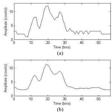
The proposed PWD method will be demonstrated here for the decomposition of observed waveform data into a series of Gaussian peaks. Figure 2(a) shows the typical example of raw backscattered waveform containing several modes. Before applying the proposed PPD method, a pre-processing is implemented to de-noise and smooth the raw signal. The result waveform is displayed in Figure 2(b), where the noise threshold
is set as 2.2 counts for this case with the threshold
N =1.1 for
the observed RIEGL full-waveform data.
(a)
(b)
Figure 2. (a)Example of the RIEGL raw backscattered signal. (b) Pre-processed result of the RIEGL raw signal example.
As shown in the Figure 2. (b), the waveform is complex, which involves multiple pulses. We compute the peak detecting threshold Cthreshold as 6 counts with =3. Actually, letting =3 is a conservative choice in order to void the wrong detection with some weak pulse close to the noise level. However, a small value of makes it possible to detect weak pulses corresponding to partially occluded targets or objects within noise at cost of reliability reducing, e.g. a low amplitude International Archives of the Photogrammetry, Remote Sensing and Spatial Information Sciences, Volume XXXVIII-5/W12, 2011
pulse detection corresponding to the ground within the topographical mapping in thick forest area.
The first global maximum amplitude value from the smoothed waveform is detected in Figure 3(a). In order to isolate the consecutive inflection points of the peak, the range coefficient W is recommend as 5to 8 bins and we use 6 bins to the entire data. The red solid line canopy curve in the Figure 3 is the fitted Gaussian peak.
After subtracting the detected single Gaussian peak from the “parent” waveform, a new waveform with different structure and shape is then obtained as shown in Figure 3 (b) and (c). A new round of peak detecting and fitting is repeated on the subtracted waveform until no peak above the can be detected as shown in Figure 3(d). Three peaks are found here using the PWD method.
threshold
C
(a)
(b)
(c)
(d)
Figure 3. The demonstration of the PWD decomposition processing
3.3 Comparison of the 3D point could derived from system and PWD method
To maximize the detection rate of relevant peaks to generate a denser 3D point cloud and, finally, to extend waveform processing capabilities by fostering information extraction from the raw signal is the main aim of full-waveform decomposition.
We compare the 3D point cloud generation result using PWD method with that from the real-time hardware systems here. Numbering the detected echoes, the points form PWD method and hardware system are both recorded as listed in Table 1. The differences of the two results are also presented.
Echoes’ numbering
Points from PWD
Points from hardware
system Difference 1 1429005 1416285 12720
2 77240 50631 26609
3 10904 2036 8868
4 2762 0 2762
5 1896 0 1896
6 1736 0 1736
7 1566 0 1566
8 1087 0 1087
> 8 559 0 559
SUM 1526755 1468952 57803
Table 1. Comparison of points from the hardware system and PWD method decomposition
From Table 1, the following conclusions can be drew: 1) the proposed PWD method can accurately recover a larger number of echoes than embedded real-time systems, and 2) the detection ability of PWD to the multiple echoes is obviously stronger with distinctive nuance in vertical structure, which will bring benefit to the computation of the forest parameters estimation, urban modelling, as well as the Terrain break lines extraction.
3.4 Contributions of PWD method
The proposed PWD method can make two important contributions: First, it makes up the weakness of the existing full-waveform decomposition method, i.e., on the one hand, there is no initialization and iteration limitation which is required in the classic Gaussian decomposition; on the other hand, besides the accurate range measurement and peak number determination, additional information about the target can be provided through the modelling parameters whereas the pulse detection method such as ASDF totally omits these parameters. This leads to a fast and effective decomposition and to richer parameter information providing for further analysis. Second, by offering a flexible coefficient setting, it gives more control to an end user in the PWD processing of the LiDAR signal (see Section 3.2).
4. APPLICATIONS OF PWD RESULTS
Figure 4. 3D point cloud section of urban area derived from the full-waveform data using PWD method
With the PWD method, a 3D point cloud has been generated as International Archives of the Photogrammetry, Remote Sensing and Spatial Information Sciences, Volume XXXVIII-5/W12, 2011
displayed in Figure 4. Despite of the derived 3D point cloud, the full-waveform decomposition steps also obtain their parameters contain significant information on the roughness, slope and reflectivity of the hit surfaces. A parametric analysis of the processed PWD full-waveform results instead of a 3D point cloud can be applied to find features. Some special applications of the PWD parameters are presented in this section.
4.1 Remove the vegetation influence
The discrimination between the low vegetation and the ground surface which are very closely located in range has been a difficult issue of the 3D points cloud filtering. Based on the understanding of the roughness of a reflected waveform, the porous surfaces (multiple echoes at different depths, equivalent to the behaviour of trees and vegetation) could be discriminated with the smooth surface (one or two echoes if there are discontinuities). Therefore, just by estimating the peak number parameters using PWD method, the reflected waveform data with multiple echoes (larger than two) will be considered as vegetation and removed from the entire data. The derived 3D point cloud can then be free from the influence of vegetation (see Figure 5). Without the influence of vegetation above the ground surface, the filtering of a 3D point cloud can then be improved.
Figure 5. Section view of an urban area with vegetation. (a) before removing the vegetation influence (b) after removing the vegetation influence
4.2 Weaken the Building Facade Influence
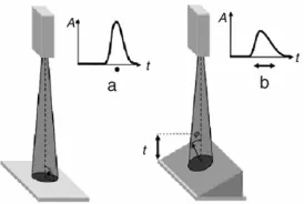
According to Jutzi and Stilla (2006), when the laser beam hits a planar surface at a certain incidence angle, the shape of the reflected waveform will change (see Figure 6).
Figure 6. (a) Waveform behavior for a laser beam hits a planar with no slope (incidence angle=0); (b) Waveform behavior for a laser beam hits a planar with a slope at a certain incidence angle
Consequently, an asymmetrical characteristic of the echoes shape may indicate the response surface as slope terrain or building facade. Furthermore, variations in the shape are also noticed with changes in the angle of incidence, i.e., the smaller the incidence angle, the narrower and more symmetrical the peak, which helps to distinguish the building façade (with narrower peak) with the slope terrain. The calculated parameter
shift
in PWD method can help to quantify the behaviour of the building façade on the return waveform. Once the building façade echo was detected, it would be cut to weaken its influence to the building remove in filtering. Figure 7 shows a example of this application.
Figure 7. Vertical view of the buildings. (a) Before the building façade weakening (b) After weakening the building façade
Abnormal altimetric points extraction 4.3
The adjacent pulses recorded in the waveform may indicate the neighborhood objects in the response surface. By analyzing the parameters of each echo and taking the relationships between adjacent waveforms into account, the abnormal altimetric points, such as the man-made structure edge, in the direction of the laser pulse travel path can be extracted (See Figure 8). In order to void the influence of vegetation, method introduced in section 4.1 can be applied first if necessary.
Figure 8.Man-made structure edge extraction results based on PWD parameters
5. CONCLUSION
A fast algorithm named progressive waveform decomposition method has been created to decompose the reflected full-waveform data form simple and complex surfaces into a series of echoes. With a superimposition of Gaussian functions, the PWD algorithm aims to detect and fit the distinct return echo components one by one using a peak detecting method. The advantages of PWD waveform processing are threefold: 1) Fast and efficient: The repeating times of the Gaussian
fitting depend on the number of the peaks of the signal, and no initialization step is needed.
2) Robust and accurate: Due to real measured value for the peak position instead of inflection points calculating, as well as the flexible coefficient setting, it is possible to fitting of asymmetric or weak echoes and then to improve the ability of peak detection. This leads to denser point clouds than the hardware system.
3) Providing with parameters: In addition to the normal Gaussian model parameters, the special peak shift parameter provides another piece of information about the shapes of the echoes. All these parameters could be useful in the analysis of waveform for different applications.
ACKNOWLEGEMENTS
The authors would like to thank reviewers of this manuscript.
REFERENCE
Baltsavias, E.P., 1999. Airborne laser scanning: Basic relations and formulas. ISPRS Journal of Photogrammetry & Remote Sensing, 54 (2-3): 199-214.
Chauve, A., Mallet, C., Bretar, F., Durrieu, S., Pierrot-Deseilligny, M., Puech, W., 2007. Processing full-waveform lidar data: Modelling raw signals. International Archives of Photogrammetry, Remote Sensing and Spatial Information Sciences, 36 (Part 3/W52), 102-107.
Hofton, M., Minster, J., Blair, J., 2000. Decomposition of laser altimeter waveforms. IEEE Transactions on Geoscience and Remote Sensing, 38 (4), 1989-1996.
Hug, C., Ullrich, A., Grimm, A., 2004. Litemapper-5600 A waveform-digitizing LIDAR terrain and vegetation mapping system. International Archives of Photogrammetry, Remote Sensing and Spatial Information Sciences, 36 (Part 8/W2), 24-29.
Jung, J. and Crawford, M., 2008. A Two-Stage Approach for Decomposition of ICESat Waveforms,” In: The International Geoscience and Remote Sensing Symposium, July 7-11, Boston, MA, III, 680-683.
Jutzi, B., Stilla, U., 2006. Range determination with waveform recording laser systems using a Wiener filter. ISPRS Journal of Photogrammetry & Remote Sensing, 61 (2), 95-107.
Mallet, C. and Bretar, F.,2009. Full-waveform topographic lidar: State-of-the-art. ISPRS Journal of Photogrammetry & Remote Sensing, 64: 1-16.
Persson, Å., Söderman, U., Töpel, J., Alhberg, S., 2005. Visualization and analysis of full-waveform airborne laser scanner data. International Archives of Photogrammetry,
Remote Sensing and Spatial Information Sciences, 36 (Part 3/W19), 103-108.
Reitberger, J., Krzystek, P., Stilla, U., 2008. Analysis of full waveform LIDAR data for the classification of deciduous and coniferous trees. International Journal of Remote Sensing, 29 (5), 1407-1431.
Roncat A., Wagner W., Melzer T., and Ulrich,A.,2008. Echo detection and localization in full-waveform airborne laser scanner data using the averaged square difference function estimator. The Photogrammetric Journal of Finnland., 21(1), 62–75.
Wagner, W., Ullrich, A., Ducic, V., Melzer, T., Studnicka, N., 2006. Gaussian decomposition and calibration of a novel small-footprint full-waveform digitising airborne laser scanner. ISPRS Journal of Photogrammetry & Remote Sensing, 60 (2), 100-112.
Wagner, W., Ullrich, A., Melzer, T., Briese, C., Kraus, K., 2004. From single pulse to full-waveform airborne laser scanners: Potential and practical challenges. International Archives of Photogrammetry, Remote Sensing and Spatial Information Sciences, 35 (Part B3), 201-206.
Zwally, H., Schutz, B., Abdalati, W., Abshire, J., Bentley, C., Brenner, A., Bufton, J., Dezio, J., Hancock, D., Harding, D., Herring, T., Minster, B., Quinn, K., Palm, S., Spinhirne, J., Thomas, R., 2002. ICESat's laser measurements of polar ice, atmosphere, ocean, and land. Journal of Geodynamics, 34 (3), 405-445.