EXTRACTION OF OPTIMAL SPECTRAL BANDS USING HIERARCHICAL BAND
MERGING OUT OF HYPERSPECTRAL DATA
A. Le Brisa∗, N. Chehatab,c, X. Briottetd, N. Paparoditisa a
Universit´e Paris-Est, IGN/SR, MATIS, 73 avenue de Paris, 94160 Saint Mand´e , France - (arnaud.le-bris, nicolas.paparoditis)@ign.fr bIRD/UMR LISAH El Menzah 4, Tunis, Tunisia
c
Bordeaux INP, G&E, EA 4592, F-33600, Pessac, France - [email protected]
dONERA, The French Aerospace Lab, 2 avenue Edouard Belin, BP 74025, 31055 Toulouse Cedex 4, France - [email protected]
KEY WORDS:Classification, Feature selection, Sensor design, Hyperspectral, Spectral bands, Multispectral
ABSTRACT:
Spectral optimization consists in identifying the most relevant band subset for a specific application. It is a way to reduce hyperspec-tral data huge dimensionality and can be applied to design specific superspechyperspec-tral sensors dedicated to specific land cover applications. Spectral optimization includes both band selection and band extraction. On the one hand, band selection aims at selecting an optimal band subset (according to a relevance criterion) among the bands of a hyperspectral data set, using automatic feature selection algo-rithms. On the other hand, band extraction defines the most relevant spectral bands optimizing both their position along the spectrum and their width. The approach presented in this paper first builds a hierarchy of groups of adjacent bands, according to a relevance criterion to decide which adjacent bands must be merged. Then, band selection is performed at the different levels of this hierarchy. Two approaches were proposed to achieve this task : a greedy one and a new adaptation of an incremental feature selection algorithm to this hierarchy of merged bands.
1. INTRODUCTION
High dimensional remote sensing imagery, such as hyperspectral imagery, generates huge data volumes, consisting of hundreds of contiguous spectral bands. Nevertheless, most of these spectral bands are highly correlated to each other. Thus using all of them is not necessary. Besides, some difficulties are caused by this high dimensionality, as for instance the curse of dimensionality or data storage problems. To answer these general problems, di-mensionality reduction strategies aim thus at reducing data vol-ume minimizing the loss of useful information and especially of class separability. These approaches belong either tofeature ex-tractionorfeature selectioncategories.
Feature extraction methods consist in reformulating and sum-ming up original information, reprojecting it in another feature space. Principal Component Analysis (PCA), Independent Com-ponent Analysis (ICA) and Linear Discriminant Analysis (LDA) are state-of-the-art feature extraction techniques.
On the opposite, feature selection (FS) methods applied toband selectionselect the most relevant band subset (among the origi-nal bands of the hyperspectral data set) for a specific problem. Furthermore, in the case of hyperspectral data, adjacent bands are very correlated to each other. Thusband extraction, that is to say the definition of an optimal set of spectral bands optimizing both their width and position along the spectra, can be consid-ered as intermediate between feature extraction techniques and individual band selection. Band selection/extraction approaches offer advantages compared to feature extraction techniques. First, they make it possible not to loose the physical meaning of the se-lected bands. Most important, they are adapted to the design of multispectral or superspectral sensors dedicated to a specific ap-plication, that is to say sensors designed to deal with specific land cover classification problems for which only a limited band sub-set is relevant.
∗Corresponding author
1.1 Feature selection
Feature selection (FS) can be seen as a classic optimization prob-lem involving both a metric (that is to say a FS score measuring the relevance of feature subsets) to optimize and an optimization strategy.
Even though hybrid approaches involving several criteria exist (Est´evez et al., 2009, Li et al., 2011), FS methods and criteria are often differentiated between “filter”, “wrapper” and “embed-ded”. It is also possible to distinguish supervised and unsuper-vised ones, whether classes are taken into account.
Filters Filter methods compute a score of relevance for each feature independently from any classifier. Some filter methods are ranking approaches : features are ranked according to a score of importance, as the ReliefF score (Kira and Rendell, 1992) or a score calculated from PCA decomposition (Chang et al., 1999). Other filters associate a score to feature subsets. In supervised cases, separability measures such as Bhattacharyya or Jeffries-Matusita (JM) distances can be used in order to identify the fea-ture subsets making it possible to best separate classes (Bruzzone and Serpico, 2000, Serpico and Moser, 2007). High order statis-tics from information theory such as divergence, entropy and mu-tual information can also be used to select the best feature subsets achieving the minimum redundancy and the maximum relevance, either in unsupervised or supervised situations: (Mart´ınez-Us´o et al., 2007) first cluster “correlated” features and then select the most representative feature of each group, while (Battiti, 1994, Est´evez et al., 2009) select the set of bands that are the most cor-related to the ground truth and the less corcor-related to each other.
De Andres, 2006) using random forests or even (Minet et al., 2010) for target detection.
Embedded Embedded FS methods are also related to a classi-fier, but feature selection is performed using a feature relevance score different from a classification performance rate. Some em-bedded approaches are regularization models associating a fit-to-data term (e.g. a classification error rate) associated to a regu-larization function, penalizing models when the number of fea-tures increases (Tuia et al., 2014). Other embedded approaches progressively eliminate features from the model, as SVM-RFE (Guyon et al., 2002) that considers the importance of the features in a SVM model. Other approaches have a built-in mechanism for feature selection, as Random Forests (Breiman, 2001) that uses only the most discriminative feature among a feature subset randomly selected, when splitting a tree node.
Another issue for band selection is the optimization strategy to determine the best feature subset corresponding to a criteria. An exhaustive search is often impossible, especially for wrappers. Therefore, heuristics have been proposed to find a near optimal solution without visiting the entire solution space. These opti-mization methods can be divided into incremental and stochastic ones.
Several incremental search strategies have been detailed in (Pudil et al., 1994), including the Sequential Forward Search (SFS) start-ing from one feature and incrementally addstart-ing another feature making it possible to obtain the best score or on the opposite the Sequential Backward Search (SBS) starting for all possible features and incrementally removing the worst feature. Variant such as Sequential Forward Floating Search (SFFS) or Sequen-tial Backward Search (SBFS) are proposed in (Pudil et al., 1994). (Serpico and Bruzzone, 2001) proposes variants of these methods called Steepest Ascent (SA) algorithms.
Among stochastic optimization strategies used for feature selec-tion, several algorithms have been used for feature selecselec-tion, in-cluding Genetic algorithms (Li et al., 2011, Est´evez et al., 2009, Minet et al., 2010), Particle Swarm Optimization (PSO) (Yang et al., 2012) or simulated annealing (De Backer et al., 2005, Chang et al., 2011).
1.2 Band grouping and band extraction
Band grouping and clustering In the specific case of hyper-spectral data, adjacent bands are often very correlated to each other. Thus, band selection encounters the question of the clus-tering of the spectral bands of a hyperspectral data set. This can be a way to limit the band selection solution space. Band cluster-ing/grouping has sometimes been performed in association with individual band selection. For instance, (Li et al., 2011) who first group adjacent bands according to conditional mutual infor-mation, and then perform band selection with the constraint that only one band can be selected per cluster. (Su et al., 2011) per-form band clustering applying k-means to band correlation ma-trix and then iteratively remove the too inhomogeneous clusters and the bands too different from the representative of the cluster to which they belong. (Mart´ınez-Us´o et al., 2007) first cluster “correlated” features and then select the most representative fea-ture of each group, according to mutual information. (Chang et al., 2011) performs band clustering using a more global criterion taking specifically into account the existence of several classes : simulated annealing is used to maximise a cost function defined as the sum, over all clusters and over all classes, of the sum of correlation coefficients between bands belonging to a same clus-ter. (Bigdeli et al., 2013, Prasad and Bruce, 2008) perform band clustering, but not for band extraction : a multiple SVM classi-fier is defined, training one SVM classiclassi-fier per cluster. (Bigdeli et
al., 2013) have compared several band clustering/grouping meth-ods, including k-means applied to the correlation matrix or an approach considering the local minima of mutual information between adjacent bands as cluster borders. (Prasad and Bruce, 2008) propose another band grouping strategy, starting from the first band of the spectrum and progressively growing it with ad-jacent bands until a stopping condition based on mutual informa-tion is reached.
Band extraction Specific band grouping approaches have been proposed for spectral optimization. (De Backer et al., 2005) de-fine spectral bands by Gaussian windows along the spectrum and propose a band extraction optimizing score based on a separabil-ity criterion (Bhattacharyya error bound) thanks to a simulated annealing. (Cariou et al., 2011) merge bands according to a cri-teria based on mutual information. (Jensen and Solberg, 2007) merge adjacent bands decomposing some reference spectra of several classes into piece-wise constant functions. (Wiersma and Landgrebe, 1980) define optimal band subsets using an analyti-cal model considering spectra reconstruction errors. (Serpico and Moser, 2007) propose an adaptation of his Steepest Ascent algo-rithm to band extraction, also optimizing a JM separability mea-sure. (Minet et al., 2010) apply genetic algorithms to define the most appropriate spectral bands for target detection. Last, some studies have also studied the impact of spectral resolution (Ade-line et al., 2014), without selecting an optimal band subset.
1.3 Proposed approach
The approach proposed in this paper consists in first building a hi-erarchy of groups of adjacent bands. Then, band selection is per-formed at the different levels of this hierarchy. Two approaches are proposed to achieve this task.
Thus, it is here intended to use the hierarchy of groups of adjacent bands as a constraint for band extraction and a way to limit the number of possible combinations, contrary to some existing ap-proaches such as (Serpico and Moser, 2007) that extract optimal bands according to JM information using an adapted optimiza-tion method or (Minet et al., 2010) that directly use a genetic algorithm to optimize a wrapper score.
2. DATA SET
The proposed algorithms were mostly tested on the ROSIS VNIR reflectance hyperspectral Pavia Center data set1. Its spectral do-main ranges from 430nm to 860nm. Its associated land cover ground truth includes the next classes : “water”, “trees”, “mead-ows”, “self blocking bricks”, “bare soil”, “asphalt”, “roofing bi-tumen” , “roofing tiles” and “shadows”.
They were also tested on the VNIR-SWIR AVIRIS Indian Pines and Salinas scenes, captured over rural areas.
3. HIERARCHICAL BAND MERGING
The first step of the proposed approach consists in building a hi-erarchy of groups of adjacent bands, that are then merged. Even though it is intended to be used to select an optimal band subset, this hierarchy of merged bands can also be a way to explore sev-eral band configuration with varying spectral resolution, that is to say with contiguous bands with different bandwidth.
3.1 Hierarchical band merging algorithm
Notations LetB ={λi}0≤i≤nbandsbe the original (ordered)
set of bands. LetH = {H(i)}
0≤i<nlevels be the hierarchy of
merged bands.H(i)={Hj(i)}1≤j≤niis the ith level of this hier-archy of merged bands. It is composed ofnimerged bands, that
is to sayniordered groups of adjacent bands fromB.
Thus, eachHj(i)is defined as a spectral domain :
Thus, the merged bandB1⊕B2obtained when merging two such
adjacent merged bandsB1andB2isB1⊕B2= [B1.λmin;B2.λmax]
LetJ(.)be the score that has to be optimized during the band merging process.
The proposed hierarchical band merging approach is a bottom-up one. The algorithm is defined below :
Initialization :H(0)=B(that is to say that merged band of the first level of the hierarchy only contains one individual original band).
Band merging : create level l+1 from level l :
Find the pair of adjacent bands at levellthat will optimize the score if they are merged : findˆk=argminkJ(T(H(l), k))with
A tableLll+1is defined to link the different merged bands at
con-secutive hierarchy levels :
Several optimization scoresJ can be examined. (In the algo-rithm described in section 3.1, this score is aimed to be mini-mized.) They can be either supervised or unsupervised, depend-ing whether classes are considered or not at this step.
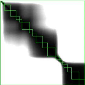
3.2.1 Correlation between bands Between band correlation (either the classic normalized correlation coefficient or mutual in-formation) (see figure 1) measures the dependence between bands. So a first band merging criterion intends to merge adjacent bands considering how they are correlated to each other. Thus, it tries to obtain consistent groups of adjacent correlated bands. Such measure inspired from (Chang et al., 2011) can be defined by next function (intended to be minimized):
J(H(l)) =Pnl
3.2.2 Spectra approximation error Band merging could also use (Jensen and Solberg, 2007)’s method to decompose some ref-erence spectra of several classes into piece-wise constant func-tions (fig. 2). Adjacent bands are then merged trying to minimize the reconstruction error between the original and the piece-wise constant reconstructed spectra.
Figure 1: Examples of groups of bands superimposed on the be-tween band correlation matrix (for Pavia data set)
Figure 2: On the left, examples of merged bands superimposed on the original reference spectra. On the right, piece-wise constant reconstructed spectra for these merged bands (Pavia data set)
3.2.3 Separability Another criterion to merge adjacent band is their contribution to separability between classes. Possible sep-arability measures are the Bhattacharyya distance (B-distance) or the Jeffries-Matusita distance (Bruzzone and Serpico, 2000, Ser-pico and Moser, 2007).
The Bhattacharyya separability between classesiandjis defined as
covariance matrix of classiradiometric distribution. As Bhat-tacharyya separability is defined for binary problems, its mean over all possible pairs of classes can be used as a global separa-bility measure.
Jeffries-Matusita measure forcclasses is then defined asJ M = Pc−1
i=1
Pc
j=i+1(1−e
−Bi;j).
At a level of the band merging hierarchy, the best set of merged bands is the one that maximizes class separability. So a possi-ble criterionJ(to minimize) for band merging can be defined as J(H(l)) =
−J M(H(l))
3.3 Results
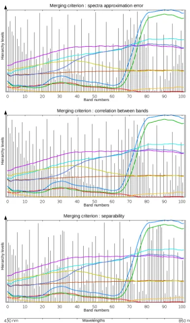
can be understood considering the underlying criteria ; indeed adjacent bands are not very correlated to each other in this do-main and the slope of spectra is strong for vegetation classes, and thus they not be merged easily according to correlation or spec-tra approximation error band merging criteria. On the opposite, the only interesting information for classification (e.g. for class separability) is the fact there is a slope there and thus the values of the bands before and after this domain. Thus, merging these red-edge bands will have little impact on class separability.
Figure 3: Hierarchies of merged bands obtained for different cri-teria for Pavia data set: spectra piece-wise approximation error (top), between band correlation (middle) and class separability (bottom). x-axis corresponds to the band numbers/wavelengths. y-axis corresponds to the level in the band merging hierarchy (bottom : finest level with original bands, top : only a single merged band). Vertical black lines are the limits between merged bands : the lower in the hierarchy, the more merged bands. Ref-erence spectra of the classes are displayed in colour.
As the hierarchy of merged bands can also be a way to explore several band configuration with varying contiguous bands with different spectral resolution, the different band configurations cor-responding to the different levels were evaluated using a classifi-cation quality measure. Thus, for each level, a classificlassifi-cation was performed using a support vector machine (SVM) classifier with a radial basis function (rbf) kernel and evaluated. Its Kappa coef-ficient was considered.
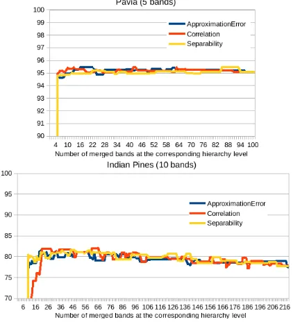
Such results are presented on figure 4. It can be seen that some spectral configurations made it possible to obtain better results than at original spectral resolution. Configurations obtained us-ing the correlation coefficient are generally less good than for the two other criteria. Except for Pavia, the spectra piece-wise approximation error merging criterion tends to lead to the best
results. But for Pavia, the classification Kappa reached using the different criteria remained very similar.
Figure 4: Kappa (in %) reached by a rbf SVM for the different band configurations of the hierarchy (x-axis = number of merged bands in the spectral configuration corresponding to the hierarchy level), for Pavia (top), Indian Pines (middle) and Salinas (bottom) data sets.
4. BAND SELECTION USING A GREEDY METHOD
To optimize spectral configuration for a limited number of merged bands, a greedy approach was first used : it performed band se-lection at the different levels of the hierarchy of merged bands, paying no attention at results obtained at the previous level. Thus a set of merged bands was selected at each level of the hierarchy. The feature selection (FS) score to optimize was the Jeffries-Matusita separability measure. It was optimized at each level of the hierarchy using an incremental optimization heuristic called Sequential Forward Floating Search (SFFS) (Pudil et al., 1994) and reminded below in its general formulation.
4.1 Sequential Forward Floating Search
It is intended to select less thanpfeatures among a feature setB. LetSbe the selected band subset andJthe FS score to maximize.
Initialization :Find bandbinBsuch thatb=argmaxz∈BJ({z})
S← {b}
J1←J(S)
While#S < p
Find bandb∈B\Ssuch thatS∪ {b}maximizes the FS score, i.e.b=argmaxz∈B\SJ(S∪ {z})
S←S∪ {b}
QuestionS: find bands∈Ssuch thatS\ {s}maximizes FS score, i.e.s=argmaxz∈SJ(S\ {z}). This means thatsis less
important than the other bands ofS, since removing it decreases the FS score less.
ifs=b Jn←J(S)
n←n+ 1 else
S←S\ {s} whileJ(S)> Jn−1
n←n−1
Jn←J(S)
QuestionS: find bands∈Ssuch thatS\ {s}maximizes FS score, i.e.s=argmaxz∈SJ(S\ {z}).
endwhile endif endwhile
Figure 5: Pavia data set: selected bands at the different levels of the hierarchy using the greedy approach for hierarchies of merged bands obtained using different band merging criteria : spectra piece-wise approximation error (top), between band correlation (middle), class separability (bottom). x-axis corresponds to the band numbers/wavelengths. y-axis corresponds to the level in the band merging hierarchy (bottom : finest level with original bands, top : only a single merged band).
4.2 Results
Obtained results on Pavia data set are presented on figure 5 : 5 merged bands (as in (Le Bris et al., 2014)) were selected at each level of the hierarchy of merged bands. It can be seen that the positions of the selected merged bands don’t change a lot when climbing the hierarchy, except when reaching the lowest spectral resolution configurations. It can also be noticed that at some level of the hierarchy the position of some selected merged bands can move and then come back to its initial position when climbing the hierarchy.
Thus, it can be possible to use the selected bands at a levellto initialize the algorithm at next levell+ 1. This modified method will be presented in section 5..
The merged band subsets selected at the different levels of the hi-erarchy were evaluated according to a classification quality mea-sure. As in previous section, the Kappa coefficient reached by a rbf SVM was considered. Results for Pavia and Indian Pines data sets can be seen on figure 6. At each level of the hierarchy, 5 bands were selected for Pavia, and 10 bands for Indian Pines. It can be seen that these accuracies remain very close to each other whatever the band merging criterion used, and no band merg-ing criterion tend to really be better than the other ones. Results obtained using merged bands are generally better than using the original bands.
Figure 6: Kappa (in %) reached for rbf SVM classification for merged band subsets selected at the different levels of the hier-archy for Pavia and Indian Pines data sets using the greedy FS algorithm (x-axis = number of merged bands in the spectral con-figuration corresponding to the hierarchy level).
5. TAKING INTO ACCOUNT THE BAND MERGING
HIERARCHY DURING FEATURE SELECTION
5.1 Algorithm
Original bands Greedy SFFS Adapted SFFS Pavia (5 bands)
Kappa (%) 95.05 95.45 95.44
Computing times 2min 1h10min 9min
Indian Pines (10 bands)
Kappa (%) 77.69 81.41 81.21
Computing times 4min 7h 40min
Figure 7: Computing times and best Kappa coefficients reached on Pavia (for a 5 band subset) and Indian Pines (for a 10 band subset) data sets for band merging criterion “spectra piece-wise approximation error”
to the greedy approach, this new algorithm uses the band subset selected at the previous lower level when performing band selec-tion at a new level of the hierarchy of merged bands.
This algorithm is described below : LetS(l)=S(l)
i 1≤i≤pbe the set of selected merged bands at level
lof the hierarchy. (NB : The same numberpof bands is selected at each level of the hierarchy.)
Initialization : standard SFFS band selection algorithm is ap-plied to the base levelH(0)of the hierarchy
Iterations over the levels of the hierarchy :
GenerateS(l+1)fromS(l): S(l+1)←Ll+1
l (S
(l)
i )1≤i≤p
Remove possible duplications fromS(l+1) if#S(l+1)< p,
finds=argmaxb∈H(l+1)\S(l+1)J(S(l+1)∪b
S(l+1)
←S(l+1);s
endif
QuestionS(l+1): find bands∈S(l+1)such thatS(l+1)\ {s}
maximizes FS score, i.e.s=argmaxz∈S(l+1)J(S(l+1)\ {s}).
S(l+1)←S(l+1)\s
Then apply classic SFFS algorithm until#S(l+1)=p.
5.2 Results
Obtained results on Pavia scene for the band merging criterion “spectra piece-wise approximation error” are presented on figure 8 : 5 merged bands were selected at each level of the hierarchy, starting from an initial solution obtained at the bottom level of the hierarchy.
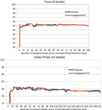
As for previous experiments, obtained results were evaluated both for Pavia (5 selected bands) and Indian Pines (10 selected bands) data sets. Kappa reached for rbf SVM classification for merged band subsets selected at the different levels of the hierarchy (built for band merging criterion “spectra piece-wise approximation er-ror”) can be seen both for the greedy FS algorithm and for the hierarchy aware one on figure 9 : obtained results remain very close, whatever the optimization algorithm.
It can be said from table 7 that both algorithms lead to equivalent results considering classification performance while the proposed hierarchy aware algorithm is really faster.
6. CONCLUSION
In this paper, a method was proposed to extract optimal spec-tral band subsets out of hyperspecspec-tral data sets. A hierarchy of merged bands was first built according to a band merging cri-terion. It was then used to explore the solution space for band extraction : band selection was then performed at each level of the hierarchy, either using a greedy approach or an adapted hier-archy aware approach. Classification results tend to be slightly improved when using merged bands, compared to a direct use of the original bands. Besides, in the context of band optimization for sensor design, it can also be a way to get more photons.
Figure 8: Pavia data set: selected bands at the different levels of the hierarchy using the proposed hierarchy aware algorithm for a hierarchy of merged bands obtained using spectra piece-wise approximation error band merging criteria
Figure 9: Kappa (in %) reached for rbf SVM classification for merged band subsets selected at the different levels of the hier-archy (built for band merging criterion “spectra piece-wise ap-proximation error”) for Pavia and Indian Pines data sets, using the hierarchy aware band selection algorithm.
Further work will investigate band optimization aiming at select-ing merged bands at different levels of the hierarchy.
REFERENCES
Adeline, K., Gomez, C., Gorretta, N. and Roger, J., 2014. Sensi-tivity of soil property prediction obtained from vnir/swir data to spectral configurations. In: Proc. of the 4th International Sym-posium on Recent Advances in Quantitative Remote Sensing: RAQRS’IV.
Battiti, R., 1994. Using mutual information for selecting features in supervised neural net learning. IEEE Transactions on Neural Networks.
Bigdeli, B., Samadzadegan, F. and Reinartz, P., 2013. Band grouping versus band clustering in svm ensemble classification of hyperspectral imagery. Photogrammetric Engineering and Re-mote Sensing 79(6), pp. 523–533.
Breiman, L., 2001. Random forests. Machine Learning 45(1), pp. 5–32.
Bruzzone, L. and Serpico, S. B., 2000. A technique for feature selection in multiclass problem. International Journal of Remote Sensing 21(3), pp. 549–563.
Cariou, C., Chehdi, K. and Le Moan, S., 2011. Bandclust: an un-supervised band reduction method for hyperspectral remote sens-ing. IEEE Geoscience and Remote Sensing Letters 8(3), pp. 565– 569.
Chang, C.-I., Du, Q., Sun, T.-L. and Althouse, M., 1999. A joint band prioritization and band-decorrelation approach to band se-lection for hyperspectral image classification. IEEE Transactions on Geoscience and Remote Sensing 37(6), pp. 2631–2641.
Chang, Y.-L., Chen, K.-S., Huang, B., Chang, W.-Y., Benedik-tsson, J. and Chang, L., 2011. A parallel simulated annealing approach to band selection for high-dimensional remote sensing images. IEEE Journal of Selected Topics in Applied Earth Ob-servations and Remote Sensing 4(3), pp. 579–590.
De Backer, S., Kempeneers, P., Debruyn, W. and Scheunders, P., 2005. A band selection technique for spectral classification. IEEE Geoscience and Remote Sensing Letters 2(3), pp. 319–232.
D´ıaz-Uriarte, R. and De Andres, S. A., 2006. Gene selection and classification of microarray data using random forest. BMC bioinformatics 7(3), pp. 1–13.
Est´evez, P. A., Tesmer, M., Perez, C. A. and Zurada, J. M., 2009. Normalized mutual information feature selection. IEEE Transac-tions on Neural Networks 20(2), pp. 189–201.
Guyon, I., Weston, J., Barnhill, S. and Vapnik, V., 2002. Gene selection for cancer classification using support vector machines. Machine Learning 46, pp. 289–422.
Jensen, A.-C. and Solberg, A.-S., 2007. Fast hyperspectral fea-ture reduction using piecewise constant function approximations. IEEE Geoscience and Remote Sensing Letters 4(4), pp. 547–551.
Kira, K. and Rendell, L., 1992. A practical approach to feature selection. In: Proceedings of the 9th International Workshop on Machine Learning, pp. 249–256.
Le Bris, A., Chehata, N., Briottet, X. and Paparoditis, N., 2014. Identify important spectrum bands for classification using impor-tances of wrapper selection applied to hyperspectral. In: Proc. of the 2014 International Workshop on Computational Intelligence for Multimedia Understanding (IWCIM’14).
Li, S., Wu, H., Wan, D. and Zhu, J., 2011. An effective feature selection method for hyperspectral image classification based on genetic algorithm and support vector machine. Knowledge-based Systems 24, pp. 40–48.
Mart´ınez-Us´o, A., Pla, F., Mart´ınez Sotoca, J. and Garc´ıa-Sevilla, P., 2007. Clustering-based hyperspectral band selection using in-formation measures. IEEE Transactions on Geoscience and Re-mote Sensing 45(12), pp. 4158–4171.
Minet, J., Taboury, J., Pealat, M., Roux, N., Lonnoy, J. and Fer-rec, Y., 2010. Adaptive band selection snapshot multispectral imaging in the vis/nir domain. Proceedings of SPIE the Interna-tional Society for Optical Engineering 7835, pp. 10.
Prasad, S. and Bruce, L. M., 2008. Decision fusion with confidence-based weight assignment for hyperspectral target recognition. IEEE Transactions on Geoscience and Remote Sens-ing 46(5), pp. 1448–1456.
Pudil, P., Novovicova, J. and Kittler, J., 1994. Floating search methods in feature selection. Pattern Recognition Letters 15, pp. 1119–1125.
Serpico, S. B. and Bruzzone, L., 2001. A new search algo-rithm for feature selection in hyperspectral remote sensing im-ages. IEEE Transactions on Geoscience and Remote Sensing 39, pp. 1360–1367.
Serpico, S. B. and Moser, G., 2007. Extraction of spectral chan-nels from hyperspectral images for classification purposes. IEEE Transactions on Geoscience and Remote Sensing 45(2), pp. 484– 495.
Su, H., Yang, H., Du, Q. and Sheng, Y., 2011. Semisuper-vised band clustering for dimensionality reduction of hyperspec-tral imagery. IEEE Geoscience and Remote Sensing Letters 8(6), pp. 1135–1139.
Tuia, D., Volpi, M., Dalla Mura, M., Rakotomamonjy, A. and Flamary, R., 2014. Automatic feature learning for spatio-spectral image classification with sparse svm. IEEE Transactions on Geo-science and Remote Sensing 52(10), pp. 6062–6074.
Wiersma, D. and Landgrebe, D., 1980. Analytical design of mul-tispectral sensors. IEEE Transactions on Geoscience and Remote Sensing GE-18(2), pp. 180–189.
Yang, H., Du, Q. and Chen, G., 2012. Particle swarm optimization-based hyperspectral dimensionality reduction for urban land cover classification. IEEE Journal of Selected Top-ics in Applied Earth Observations and Remote Sensing 5(2), pp. 544–554.