MULTIDIMENSIONAL ROUGHNESS CHARACTERIZATION FOR MICROWAVE
REMOTE SENSING APPLICATIONS USING A SIMPLE PHOTOGRAMMETRIC
ACQUISITION SYSTEM
Philip Marzahn1, Dirk Rieke-Zapp2, Urs Wegmuller3and Ralf Ludwig1
1
Department of Geography Ludwig-Maximilians University of Munich Luisenstrasse 37, 80333 Munich, Germany [email protected]
2
Institute of Geological Science University of Bern
Baltzerstrasse 1+3, CH-3012 Bern, Schwitzerland 3
Gamma Remote Sensing
Worbstr. 225, CH-3073 Guemlingen, Schwitzerland Commission V/6
KEY WORDS:Soil Surface Roughness, Photogrammetry, SAR, Directional Scattering, Detrending, Statistics
ABSTRACT:
Soil surface roughness, as investigated in this study, is a critical parameter in microwave remote sensing. As soil surface roughness is treated as a stationary single scale isotropic process in most backscattering models, the overall objective of this study was to better understand the role of soil surface roughness in the context of backscattering. Therefore a simple photogrametric acquisition setup was developed for the characterization of soil surface roughness. In addition several suited SAR images of different sensors (ERS-2 and TerraSAR-X) were acquired to quantify the impact of soil surface roughness on the backscattered signal. Major progress achieved in this work includes the much improved characterization of in-field soil surface roughness. Good progress was also made in the understanding of backscattering from bare surface in the case of directional scattering.
1 INTRODUCTION
Micro scale soil surface roughness is a critical parameter in a wide range of environmental applications. In microwave remote sensing, it is well known that micro scale soil surface rough-ness has a considerable impact on the backscatter signal. With-out considering roughness terms in several retrieval algorithms, the derivation of geo-physical variables will lead to insufficient results or in a general over- or underestimation of the desired variables. Despite this, recent studies have shown, the periodical component of soil surface roughness and its orientation cause sig-nificant backscatter differences in different SAR images acquired with short temporal intervals under slightly different aspect an-gles (Wegmuller et al., 2011). However, for an appropriate char-acterization ofin-situsoil surface roughness measurements, the default measurement devices are still not sufficient in accuracy (mesh boards) or in the acquisition speed (laser profiler). Thus, precise roughness measurements with a statistically robust acqui-sition size are so far rarely available, leading to a generalized roughness representation in recent backscatter models. In such models, soil surface roughness is generally treated as single scale stationary isotropic process. Indeed, as soil surface roughness in an agricultural environment can be considered as multi-scale and anisotropic, a three-dimensional acquisition scheme is required to accomplish theses requirements (Marzahn et al., 2012a,b). In this paper we present a simple acquisition setup to acquire soil surface roughness and show the impact of soil surface roughness on microwave backscattering from agricultural fields in the spe-cial case of directional scattering. Datasets were acquired at the Wallerfing test site, which is part of the SMOS Cal/Val Upper Danube test site (Schlenz et al., 2010).
2 METHODS
Several field campaigns were scheduled in conjunction with ERS-2 and TerraSAR-X acquisitions over the Wallerfing test site which is part of the SMO Cal/Val activities (Schlenz et al., 2010) located in the Upper Danube watershed approx. 100 km northeast of Mu-nich. The region, which has a low relief energy, is mainly agri-cultural in character and the main crops are winter wheat, win-ter barley, corn and sugar beet. During the campaign most of the crops had been sown already and were already at the beginning of their growth. The seedbed structure was at all sample points still well developed due to the lack of precipitation. Thus, the sample points (elementary sample units, ESU) all represent an already prepared seedbed pattern. Table 1 summarizes the characteris-tics of the sample points. In addition to the roughness measure-ments, soil moisture, vegetation height and coverage, row orien-tation and linearity as well as row distance were measured. For the entire test site a landuse map was available.
2.1 Roughness Acqusition Setup
align fixture
imagery
frame frame
overlap
Figure 1: Roughness acquisition scheme and image arrangement for stereo coverage of the frame
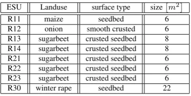
ESU Landuse surface type size m2
R11 maize seedbed 6
R12 onion smooth crusted 6 R13 sugarbeet crusted seedbed 8 R14 sugarbeet crusted seedbed 8 R21 sugarbeet crusted seedbed 6 R22 sugarbeet crusted seedbed 6 R23 sugarbeet crusted seedbed 6 R30 winter rape seedbed 22
Table 1: Characteristics of sample points acquired within this study
al. (2012a). As LPS needs for establishing the exterior orientation
Ground Control Points(GCPs), a reference frame in the size of 1 x 2.5 m2was built providing 28 GCPs with a vertical accuracy of 0.1 mm measured with a caliper ruler. As the frame is lim-ited in its size, it is necessary, for larger roughness acquisitions, to acquire consecutive image acquisitions of the frame by mov-ing it along a levelled plane which is ensured by an align fixture (see Fig. 1). During post processing, the individual DSMs were merged to a final large DSM by image matching techniques. In this study, roughness measurements were made over several bare or sparse vegetated fields. Over the latter ones, the vege-tation was carefully removed from the scene without disturbing the soil’s surface. For each sample point acquisitions were made parallel and perpendicular to the row direction of the agricul-tural fields. Table 1 summarizes the characteristics of the sample points where soil surface roughness was measured.
2.2 Roughness Characterization
Soil surface roughness can be characterised by a vertical and a horizontal component. Thus, to quantify soil surface roughness, two different roughness indices where chosen to numerically de-scribe soil surface roughness. To quantify the vertical component, the RMS heightswas chosen, which is defined as:
s[cm] =
and describes the standard deviation of the heights(Z)to a ref-erence height Z
. The horizontal roughness component is de-scribed by the autocorrelation lengthl. For an efficient estimation ofl, a variogram analysis was used and inverted the autocorrela-tion funcautocorrela-tion (ACF) from a calculated theoretical direcautocorrela-tional var-iogramγ˜h~j
, wherelis defined as the distance (h) at which the ACF drops undere−1(Blaes and Defourny, 2008). This
im-plies an exponential fit of the theoretical variogram and therefore
of the ACF.
The theoretical variogram(˜γ)with an exponential shape is fit-ted to a directional experimental variogram
defined as (Webster and Oliver, 2007):
ˆ
From the theoretical variogram(˜γ)the ACF(˜ρ)can be derived as follows:
˜
ρ(h) = 1− ˜γ(h) ˜
γ(∞) (3)
where˜γ(h)is the semi variance at distancehbetween two points and˜γ(∞)is the semi variance at distance where the sill of the variogram is reached. For the assumed exponential model, where the sill is asymptotically approached,˜γ(∞)corresponds to the distance where 95 % of the sill is reached (Blaes and Defourny, 2008).
To characterize the anisotropic pattern of a corresponding soil surface, the directional autocorrelation length was calculated for direction between 45°and 135°with a 1°interval.
2.3 Decomposing Soil Surface Roughness
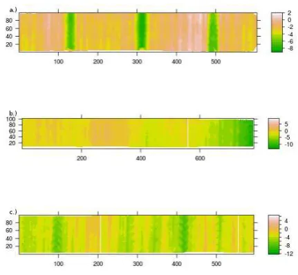
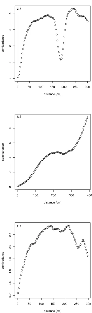
From Figure 2a and its corresponding sample variogram (Fig. 3a) it is obvious that a two scale roughness pattern can be observed on an agriculturally formed soil surface. As different roughness scales have an impact on the backscattered signal in microwave remote sensing, it is important to characterize both scales. There-fore, again variography is used to decompose and characterize the soil surface at different scales. As the variogram shows a surface inherent behaviour with strong similarities at distances in range of 180 cm, which correspond to the wheel tracks in Figure 2a, a two scale roughness pattern is indicated. Thus, the variogram for the whole sample plot describes the semi-variance of the roughness pattern which is strongly imposed by the large scale roughness pattern (e.g. wheel tracks of drilling machine). To characterize the small scale roughness pattern (e.g. seedbed rows, soil clod distribution) we defined a threshold to mask out the wheel tracks and calculated variograms for each surface again. As a result, for each roughness scale a roughness index is calculated.
2.4 Detrending
As can be seen in Figure 2b and 3b several DSMs showed a spa-tial trend in elevation due to higher order topographic patterns such as general slope effects. Lievens et al. (2009) described the importance of detrending the data and the effects of different de-trending procedures on the retrieved roughness indices. In this study, two detrending models have been defined which can be described by:
Zmod∼mX+b (4)
for the linear model and
Zmod∼b+m1X+m2X 2
+m3X 3
+...mnXn (5) for the polynominal model, wheremandbrepresent the regres-sion coefficients slope and intercept andXthe x-coordinate of the sample DSM. The detrended surfaceZresthen is defined as:
Zres=Z−Zmod (6)
2.5 SAR Data
Date Sensor Dop. Centroid[H z] Mode Pol
20110402 ERS -2427.0 Image VV
20110423 ERS 160.0 Image VV
20110426 ERS 752.0 Image VV
20110507 TSX -9.8 Stripmap VV/HV
20110514 ERS -3598.0 Image VV
20110523 ERS 7.0 Image VV
Table 2: Acquired SAR imagery and corresponding characteris-tics
R11 R12 R13 R14 R21 R22 R23 R30
0.17 0.13 0.05 0.07 0.05 0.06 0.02 0.22
Table 3: Root mean square error in cm of generated DSM height values compared to the manually measured GCPs for each sample point
the beginning of the growing season for the major crops in the test site. Table 2 summarizes the main characteristics of the ac-quisitions, while Figure 4 show as an example the backscattering in an ERS-2 image over the test site.
To detect a potential directional scattering over several agricul-tural fields, a SAR image is split into five sub looks according to Wegmuller et al. (2011) with a 50 percent overlap and HSI images are generated, where hue corresponds to the backscatter ratio of two sub looks, saturation to the backscatter change and intensity to the backscattering in the first image of the pair. Figure 5 shows as an example a HSI composite for the 23 of May 2011.
3 RESULTS AND DISCUSSION
3.1 Roughness characterization
Table 3 shows the root mean square error in the Z-direction (RMSEZ)
of the sample plots. The results show a high accuracy of the gen-erated DSMs compared to the manually measured checkpoints installed on the reference frame, thus providing a robust basis for the characterization of soil surface roughness statistics.
Figures 2 and 3 show as an example three generated DSM with typical problems occurring when measuring soil surface rough-ness in an agricultural environment. All DSMs show a multi scale roughness pattern ranging from small (micro) scale roughness pattern comprising the soil clods and seedbed rows over meso scale roughness (wheel tracks) and large scale roughness pattern such as general slope effects. Table 4 summarizes the character-ization of the roughness spectra by using the defined roughness indices for the micro (s1andl1) and the meso roughness scale (s2 andl2) separately and the output from the detrending procedure. By analysing the effects of detrending it is obvious that for the RMS height no significant change is observed due to the detrend-ing procedure. Results for the autocorrelation lengthlchange significantly in the order of several decimetres. Except for R30, a 22 m2large sample plot, a significant change inscan be observed,
due to the strong topographic influence with a range in heights of 20 cm. To model this strong trend a polynomial approach of 9th order was chosen.
Figure 3a indicates a significant two-scale roughness pattern for sample plot R12. Different points with a certain distance in range of 200 cm to each other show a strong similarity, thus indicating periodicity in the soil surface roughness pattern with a range of 200 cm. From Figure 2a it is obvious that this pattern is clearly related to the wheel tracks of the tillage machines used during
Figure 2: Three sample DSMs of different roughness plots show-ing a.) a significant two scale roughness pattern (R12), b.) a spatial trend (R14) and c.) no spatial trend with an insignificant two scale roughness pattern (R21). Units in cm
ESU s1 s2 l1 l2
R11 0.88 1.84 11.0 29.5
R12 0.85 1.73 71.6 38.27
R13 1.15 (1.09) 2.43 (2.84) 38.3 (17.7) 53.04 (69.05) R14 0.24 (0.86) 2.26 (2.5) 41.01 (96.39) 98.04 (169.14)
R21 1,24 1.45 31.1 38.52
R22 0.77 (0.93) 1.12 (1.51) 20.5 (26.4) 23.47 (55.4) R23 1.08 (1.31) 2.38 (2.71) 27.3 (25.7) 105.6 (107.5) R30 1.18 (2.84) 1.19 (3.26) 17.2 (145.7) 17.2 (359.52)
a.)
b.)
c.)
Figure 3: Sample variograms of the roughness plots from Fig 2 showing a.) a significant two scale roughness pattern (R12), b.) a spatial trend (R14) and c.) no spatial trend with an insignificant two scale roughness pattern (R21)
Figure 4: ERS-2 scene, acquired at the 23 of May 2011, over the Wallerfing test site, indicating strong directional backscattering over several fields in the north-western part of the image
seedbed preparation. Thus the sharply bounded wheel tracks with a height difference of 4-6 cm to the surrounding seedbed biases the characterization of the roughness indices. All sample plots show this two scale roughness representation, due to the avail-ability of a seedbed structure imposed over wheel tracks, at which for the small scale roughness pattern the values fors1andl1are lower than for the large scale roughness pattern. For sample plot R12, which represents a smooth crusted onion field, the auto-correlation length for the small scale roughness pattern is higher than the large scale roughness pattern, indicating a very smooth surface with sharply bounded wheel tracks (Fig. 2a). It should be highlighted, that even under the same land use type (e.g. sugar beet) the roughness values indicate different roughness condi-tions, which are a result of the different tillage machines used and the state of crusting. Sample plots R14 and R21 illustrate this effect, both represent sugar beet fields at the same crusted stage. In contrast, sample plot R30 shows no significant two scale roughness process, which is due to the missing presence of wheel tracks or other higher order roughness patterns and thus rough-ness is only defined by the present seedbed structure. As a result, the values ofsandlare equal for both scales.
3.2 SAR data and the identifying of directional scattering
Figure 4 reveals a strong backscatter for several fields in the north-western part of the scenes, indicating either vegetated fields as well as man made structures or directional scattering from bare fields (Wegmuller et al., 2011). The HSI image with an Doppler difference of 1000 Hz, which correspond to a difference in the look vector of 0.5°, indicate that those fields are characterized by directional scattering. Those fields are mostly bare recently seedbed prepared or sparsely vegetated fields, with the row pat-tern orientated quasi perpendicular to the sensors look vector with a difference of±5°. Wegmuller et al. (2011) found similar obser-vations over the Flevoland test site. Comparing those fields with the neighbouring fields, with a different row orientation but same landuse type and phenology, the backscattering is up to 10 dB higher. Thus, a directional backscattering, which mainly origi-nates from the row orientation can be observed, however there are several differences between different fields (see Fig. 4) which only differ in the observed roughness conditions.
3.3 Impact of soil surface roughness on backscattering
Figure 5: HSI (HueSaturationIntensity) composite of the backscatter ratio (hue), backscatter change (saturation) and backscattering in the first image of the pair (intensity) over Wallerfing site on 23 of May 2011. Backscatter ratio (hue) ranges from 6 to + 6 dB; mean intensity (intensity) from 22 dB to + 6 dB; absolute backscatter change (saturation) from 0 to + 6 dB. Red indicates higher intensity for the sub look 1, and green higher intensity for sub look 5.
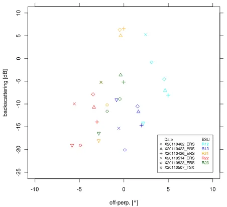
a strong first order dependency of the directional scattering from the row orientation which was also observed by Wegmuller et al. (2011). However, a secondary dependency can be observed from the roughness conditions. Thus, the first order dependency can be described by a Gaussian model (Mattia, 2011; Wegmuller et al., 2011) with a peak at rows orientated perpendicular to the sensors look vector (in Figure 6, perpendicular=0°). However, for sam-ple points R12 and R21 the backscattering is significantly higher compared to the other sample points. This could be related to the roughness conditions measured at both sample points, as both show the same roughness values for the meso scale roughness pattern with an autocorrelation length of approx. 38 cm. In con-trast, for the TSX data, no significant dependency of the direc-tional scattering from the measured roughness conditions could be observed, thus it is only dependent from the row orientation. Following the study of Lievens et al. (2009), detrending of ness measurements has a strong impact of the calculated rough-ness indices. As mentioned above, this effect is mainly present for the autocorrelation length. Indeed, the different scales of soil surface roughness, which were reduced by detrending to a sin-gle scale, have an impact on microwave backscattering. From Figure 6 one could observe that sample point R13 has a signifi-cantly lower backscatter in every SAR acquisition than samples R12 and R21, even when detrending reveals the same autocor-relation length. Looking closely to the non-detrended roughness values of R13, the surface shows a general slope and as a conse-quence lowering and disturbing the superimposition of the micro and meso scale roughness component to a comparable strong di-rectional backscatter .
4 CONCLUSIONS AND FUTURE WORK
In this paper we proposed a simple and efficient approach for measuring multi dimensional soil surface roughness in an agri-cultural environment for microwave remote sensing applications. A customized Canon EOS 5D was used to generate and pro-vide highly accurate digital surface models. With a vertical dis-placement of RMSEz ≤0.2 mm, the technique is suited for the
characterization of soil surface roughness for microwave remote sensing studies (Lievens et al., 2009). In this study we proposed an approach to decompose soil surface roughness in its different scales, ranging from micro scale (soil clods and seedbed rows)
Figure 6: Backscattering [dB] versus row direction (0°= rows per-pendicular to the sensors look vector) for the roughness sample plots
over meso scale soil surface roughness (wheel tracks) to a macro scale component (general slope, formed by the landscape). As each scale has its contributions to microwave backscattering, the effect of detrending on soil surface roughness measurements has to reconsidered. From the roughness measurements made in this study one can obtain that for the detrended data, several samples yield the same roughness values (e.g. R13) as for other sam-ples without detrending (e.g. R12/R21). However, under the same conditions (soil moisture, row orientation, phenology) the backscattering is significantly lower than for the non detrended samples, leading to the assumption that using detrended rough-ness measurements biases a potential backscatter model. Indeed, this conclusion has to be approved by further investigations. In the context of “Flashing Fields”, which are characterised by a strong directional scatter caused by the seedbed rows orienta-tion to the sensors look vector, we confirmed the investigaorienta-tions of Wegmuller et al. (2011) and Mattia (2011). However, we also identified a second order dependency of the flashing by the soil surface roughness conditions. From this study, it is to conclude that for a C-Band sensor such as ERS-2 an autocorrelation length of approx. 38 cm significantly increases the flashing effect in mi-crowave remote sensing.
Future work will comprise an in depth analysis of the effect of de-trending on roughness values and their impact on SAR backscat-ter. In addition further “Flashing Fields” will be analysed with a focus on the impact from soil surface roughness and the impact of the different roughness scales.
ACKNOWLEDGEMENTS
References
Blaes, X. and Defourny, P., 2008. Characterizing bidimen-sional roughness of agricultural soil surfaces for SAR mod-eling. Geoscience and Remote Sensing, IEEE Transactions on 46(12), pp. 4050–4061.
Lievens, H., Vernieuwe, H., Alvarez-Mozos, J., De Baets, B. and Verhoest, N., 2009. Error in radar-derived soil moisture due to roughness parameterization: An analysis based on synthetical surface profiles. Sensors 9(2), pp. 1067–1093.
Marzahn, P., Rieke-Zapp, D. H. and Ludwig, R., 2012a. Assess-ment of soil surface roughness statistics for microwave remote sensing applications using a simple photogrammetric acquisi-tion system. ISPRS Journal of Photogrammetry and Remote Sensing submitted, pp. submitted.
Marzahn, P., Seidel, M. and Ludwig, R., 2012b. Decomposing dual scale soil surface roughness for microwave remote sens-ing applications. Remote Senssens-ing submitted, pp. submitted. Mattia, F., 2011. Coherent and incoherent scattering from
anisotropic tilled soil surfaces. Waves in Random and Com-plex Media 21(2), pp. 278300.
Rieke-Zapp, D. and Nearing, M., 2005. Digital close range pho-togrammetry for measurement of soil erosion. Photogrammet-ric Record 20(109), pp. 69–87.
Rieke-Zapp, D., Tecklenburg, W., Peipe, J., Hastedt, H. and Haig, C., 2009. Evaluation of the geometric stability and the ac-curacy potential of digital cameras – comparing mechanical stabilisation versus parameterisation. ISPRS Journal of Pho-togrammetry and Remote Sensing 64(3), pp. 248–258. Schlenz, F., Dall’Amico, J., T., Loew, A. and Mauser, W., 2010.
Smos validation in the upper danube catchment (udc): A sta-tus report eigth month after launch. In: Proceedings of ESA LIving Planet Symposium 2010 Bergen, Norway.
Webster, R. and Oliver, M. A., 2007. Geostatistics for Environ-mental Scientists. 2 edn, John Wiley /& Sons, LTD.