Effects of chemical reactions on iterative
methods for implicit time stepping
G. J. S. Leeming
a, K. U. Mayer
b& R. B. Simpson
c ,*
aDepartment of Applied Mathematics, University of Waterloo, Waterloo, Ontario, Canada N2L 3G1 b
Department of Earth Sciences, University of Waterloo, Waterloo, Ontario, Canada N2L 3G1 c
Department of Computer Science, University of Waterloo, Waterloo, Ontario, Canada N2L 3G1
(Received 3 September 1997; accepted 1 June 1998)
We compare the performance of the fully coupled Newton–Raphson method with the sequential iteration approach (SIA) for solving the implicit time stepping equations of reactive transport modeling. We formulate the implicit time stepping equations for a demonstration model that incorporates homogeneous equilibrium reactions, i.e. carbonate hydrolysis, and a heterogeneous equilibrium reaction, i.e. the dissolution/precipitation of calcite. The demonstration model uses a coupled pair of mixing cells as a simplified form of transport. The effects of the homogeneous and heterogeneous reactions on the iterative methods are demonstrated.q1998 Elsevier Science Limited. All rights reserved
Keywords: reaction–transport, SIA, iteration, Newton’s method, precipitation, carbonate hydrolysis.
1 INTRODUCTION
When physical transport processes are slow relative to chemical reaction rates, it is common to model the transport dynamically and to model the chemistry as being in quasi-equilibrium at each instant of time. After spatial discretiza-tion, the mathematical equations for the model then form a differential algebraic system, with differential equations for the dynamic processes and algebraic equations for the quasi-equilibrium processes. These equations are typically approximated by algebraic systems using implicit time step-ping, and solved numerically. In this paper, we demonstrate how transitions in chemical quasi-equilibrium states and dissolution/precipitation affect the convergence of iteration strategies for solving these algebraic systems.
There are two, in some senses competing, strategies for solving these non-linear equations. One of these is based on the use of the Newton–Raphson method applied to the full system, which we will refer to as global linearization. The other general approach is operator splitting, in which the equations are partitioned into a subsystem that couples the spatial discretization cells by their transport mechanism and a subsystem for calculating the chemical speciation in each
cell separately. In this paper, we study the particular version of operator splitting referred to as the sequential iteration approach (SIA). The Newton–Raphson (hereafter shortened to Newton) method can also be used in SIA for solving the subsystems that arise from the operator splitting. An alter-native operator splitting technique that uses a level of trans-port–reaction coupling that is intermediate between global linearization and SIA has been presented by Barry et al.1 Details of the implicit time stepping equations and these solution methods are presented in Section 3.
To enable us to compare details of the performance of these methods, we use a small demonstration model which incorporates both homogeneous and heterogeneous reac-tions, and which exhibits some of the problems which are typical for large-scale reaction–transport modeling. Although the equations of our micro-model are simplified versions of those used in realistic modeling, we believe they adequately capture the aspects of these phenomena that affect the computational methods being studied. Using this system, we demonstrate the influence of these reactions on SIA and global linearization, we study modifications of the Newton method that ensure non-negative values of con-centration iterates, and we look briefly at the performance of the public domain DAE code, DASSL.3
A pair of coupled mixing cells is used to incorporate
Printed in Great Britain. All rights reserved 0309-1708/98/$ - see front matter
PII: S 0 3 0 9 - 1 7 0 8 ( 9 8 ) 0 0 0 1 9 - 0
333
elementary physical transport into the demonstration. The reaction component of our demonstration example is the well-known carbonate system (e.g., Stumm and Morgan18) involving the dissociation of carbonic acid to bicarbonate and subsequently to the carbonate ion as a function of pH, as well as the dissolution/precipitation of the solid phase cal-cite. Simple conventional mass action equations are used for the chemical reactions. We formulate the dissolution/preci-pitation conditions as a single algebraic equation, which we believe is a new computational formulation. This results in a uniform computational treatment of heterogeneous and homogeneous reactions.
Global linearization is widely used in complex transport modeling, including reservoir simulation and multiphase pollutant transport, groundwater modeling, partly because of its robustness in the presence of a variety of model phenomena (e.g., Forsyth6and Forsythet al.7). When it is performing well, the SIA seems to be more efficient for models involving multiphase systems and involving a large numbers of chemical species, as stated in Yeh and Tripathi19 and observed by a number of investigators, including Engesgaard and Kipp,5 Zysset et al.21 and Runkel et al.14 However, there are some questions raised about the reliability and range of effectiveness of this approach, as reported in Steefel and MacQuarrie.17SIA is also preferred for computations designed to use existing equilibrium batch models for the description of the chemical subsystem.14
The specific cases tested and performance data on the methods are presented in Section 4. We observe that the effects of ‘stiffness’ arising from the chemistry of the car-bonate species affect the Newton method in essentially the same way whether it is used in the fully coupled global linearization manner or as the inner iteration of SIA. In our demonstration system, iteration in SIA is only required if the solid phase is present. In this case, we observe that the convergence of SIA is dominated by the outer iteration, which couples each cell’s reactions to the global transport. In both of these approaches, the use of the Newton method can give rise to non-positive iterates or even con-verge to non-physical solutions of the model equations. Non-linearities in more complex models may not be able to use non-positive iterates. We discuss several techniques for modifying the use of the Newton method to avoid
non-physical values in the iterates and to speed up conver-gence. In particular, we demonstrate the effects of several update modification schemes, as an alternative to the rather costly method of basis switching (e.g., Bethke2).
In our concluding section, we note briefly that the chemistry of our test cases affects the performance of the public domain DAE code DASSL in ways comparable to the observations of Section 4, and make some conclusions and general observations.
2 THE DEMONSTRATION MODEL
For our test computations, we have taken equilibrium and transport equations which are simplified versions of model-ing equations but which we believe contain at least some of the basic computational difficulties. Simplifications include the use of unity activity coefficients and assuming iso-thermal conditions. Electrical neutrality is not necessarily enforced in our demonstration model. These simplifications have essentially no influence on the focus of this study, which is the numerical solution of the governing equations. Realistic mathematical models for multicomponent reactive transport have been discussed extensively.4,5,8–10,13,14,19–21 We describe the transport component of our demonstra-tion model using the general notademonstra-tion of a standard reactive transport formulation, (e.g., Yeh and Tripathi19 or Steefel and MacQuarrie17). We haveNS¼6 mobile dissolved spe-cies andNP¼1 immobile solid phase species (CaCO3). All NS þ NP species can be expressed in terms of NC ¼ 3 components (CO23¹, Ca2þ, Hþ) chosen from the dis-solved species.
For physical transport, we prescribe dynamic volume flow rates, vi(t) (l s¹1
), between two mixing cells, as shown in Fig. 1. These rates are taken as positive in the direction of the arrows shown in the figure. Conservation of the incompressible liquid mass requiresv0(t)¼v3(t) and
v0(t)¼v1(t)þv2(t). If 0,v1(t)#v0(t), thenv2(t).0, so the transport occurs from cell 1 to cell 2 only and it is equivalent to v1(t) ¼ v0(t). This is the situation in the classical mixing cell method, e.g., that used by Schulz and Reardon15for reactive transport modeling. In our model, we force two-way coupling between the cells by requiring
0,v0(t),v1(t), and consequentlyv2(t),0: (1)
This elementary formulation of transport is a simplification of the usual advection and diffusion processes used in finite volume or finite element modeling, maintaining the two-way coupling between adjacent cells, which allows us to focus on the computation of chemical equilibria. Its equivalence to a two-cell finite volume model for diffusion–advection transport is outlined in Appendix B. The cell concentrations are simply the number of moles in the cell divided by the cell volume. To get a uniform description of the different demonstration cases, our nota-tion is set up for a general number, Ncells, of cells. The notations for the concentrations and other cell-related
quantities are as follows.
Ti,k total concentration of componenti,i ¼1 toNC, in
cellkfor k¼1 toNcells
Tk the vector of total concentration of components in cellk¼(T1,k, T2,k, …, TNC,k)
t
Ci,k aqueous concentration of speciesi, fori¼1 toNS, in cellk
Ck the vector of aqueous concentrations of species in cellk¼(C1,k, C2,k, …, CNS,k)
t
Ti,in total aqueous concentration of componentiin solution flowing into cell 1 at flow ratev0(t),i¼1 toNC
Tin the vector of total aqueous concentrations of components in the solution flowing into cell 1 at flow ratev0(t),(T1,in, …, TNC,in)
t
Fi,k the inflow rate of the total aqueous concentration of componenti into cellk[mol s¹1
]
Fk the vector of inflow rates of total aqueous concen-trations for all components into cellk,
Fk¼(F1,k, …, FNC,k) t
hk volume of cellk[l]
All concentrations are in mol l¹1
; in the case of the solid phase,Pk, this is a bulk concentration in the sense of being the number of moles in the cell divided by the volume of the cell. We note that lower case ‘c’ is used in Ref.19for
Ci,k.
2.1 The general form of the mass balance equations and transport equations
The conservation of mass for the chemical subsystem can be described in terms of total component concentrations:
Tk¼ACkþPkb k¼1, …, Ncells, (2)
which will lead to a set ofNC mass balance equations for each cell. Eqn (2) indicates that the total component con-centrations are combinations of dissolved species and the solid phase with the stoichiometric coefficients as weights. These coefficients appear in the rows of the NC 3 NS
matrix A and in the NC vector b (see Refs. 20 or 21 and
the example below). We assume that no solid calcite is carried into cell 1 by the inflow; hence, Tin is related to the concentrations of the dissolved species in the inflow, which we could write asCi,in, byTin¼ACin, i.e. the form of
eqn (2) withPin ¼0. At this point, it should be noted that total concentrations of components have to take positive values to be physically meaningful, with the exception of Hþ, for which the mass balance equation is based on the proton condition and is therefore not required to be positive.12,17
For our Ncell ¼ 2 model of Fig. 1, the cell coupling requirement 1 implies flowv2transports solutes from cell 2 into cell 1. Hence, we can express the mass transport of the
total concentrations of components as follows:
F1(t)¼v0(t)(Tin(t)¹AC1(t))þv1(t)A(C2(t)¹C1(t))
(3)
¼v0(t)Tin(t)¹(v0(t)þv1(t))AC1(t)þv1(t)AC2(t)
F2(t)¼v1(t)AC1(t)þv2(t)AC2(t)¹v3(t)AC2(t)
¼v1(t)(AC1(t)¹C2(t)):
Combining these mass transport expressions with a conti-nuity equation yields the mass conservation equation for the physical subsystem, which can be described by a set of NcellsNCdifferential equations:
hkdTk(t)=dt¼Fk(t) fork¼1 toNcells: (4)
Since Fi,kis linear inCi,k, eqn (4) can be written as
dTk(t)=dt¼
where, in general, the coefficients in theNcells3(Ncellsþ1) matrix Vk,k9(t) describe the inter-cell flows. In this paper, withNcells ¼2, these flows are
V1,0 V1,1 V1,2
From eqns (2) and (5), we have 2NcellsNCequations for the
Ncells(NCþNSþNP) variables describing the total compo-nent concentrations forNCcomponents, plus the concentra-tions of all dissolved species and the solid phase in theNcells
cells. For a complete model description, we require addi-tional equilibrium conditions for the dissolved species and the solid phase in each cell, which provide (NSþNP¹NC)
equations for each cell, closing the system of model equations.
2.2 Specific form of the homogeneous and heterogeneous reaction equations
Species CO23¹, Ca2þand Hþhave been chosen as theNC¼
3 components plus the solvent species H2O itself. The
con-centrations of the remaining dissolved species, OH¹
, HCO3¹ and H2CO3, can be obtained based on the following NS ¹NC ¼ 3 reaction equations (7)–(9), as described in Steefel and MacQuarrie.17 The equilibrium constants for these reactions are provided in Table 1.
H2OOHþþOH¹ K3 (7)
HCO3¹OCO23¹ þHþ K1 (8)
The identification of index i for aqueous concentrations
From the law of mass action, the model equilibrium conditions for reactions (7)–(9) in the kth cell take the form
gl Ck
ÿ
¼0 forl¼1, 2, 3 (11)
for three functions of the vector argument of length 6,x¼ (x1,…,x6):
g1(x)¼K3¹x3x4 (12)
g2(x)¼K1x5¹x3x1
g3(x)¼K2x6¹x23x1:
To complete the description of our demonstration model, we require one additional equation, which describes the dissolution/precipitation reaction. The reaction equation for the mineral calcite is given by:
CaCO3(s)OCa2þþCO23¹ Ksp, (13)
with the appropriate solubility product constant given in Table 1. For each cell, we letPk be the number of moles of CaCO3(s) divided by the cell volume (assumed
constant).
The stoichiometric matrixAand vectorbof eqn (2) are
A¼
The mathematical formulation of equilibrium dissolution/ precipitation reactions is not as straightforward as for the hydrolysis reactions presented previously. In each cell, the solution may be either saturated or undersaturated with respect to the mineral. For saturated conditions, the equili-brium state is characterized by
Ksp¼C1,kC2,k andPk$0, (15)
while an undersaturated solution with no solid phase present is characterized by the inequality
Ksp.C1,kC2,kandPk¼0: (16)
We propose an equilibrium formulation incorporating con-ditions (15) and (16) into a single algebraic equation (18),
based on the function g4defined as follows:
g4(x,y,z)¼Ksp¹xyif z.0 and min(x,y)$0 (17)
¼Ksp¹xyif z¼0 andxy.Ksp and min(x,y)$0
¼0 ifz¼0 andxy#Ksp and min(x,y)$0
¼zif z,0 and min(x,y)$0
¼min(x,y)2 if min(x,y),0:
The physically meaningful regions of (x,y,z) space for con-centrations (C1,k,C2,k,Pk) are the section of the hyperboloid surface Ksp ¹xy ¼ 0 for which z$ 0 and the region of
the z ¼ 0 plane for which x . 0, y . 0 and xy , Ksp. These regions are characterized by being the zero function value sets of g4, i.e. Eqn (18) states that C1,k,C2,k andPk
must lie in the physically meaningful regions of (x,y,z) space:
g4(C1,k, C2,k, Pk)¼0: (18)
The function values ofg4(x,y,z) for non-physical values of arguments x,y,z are relatively arbitrary non-zero values chosen to provide some degree of continuity at the bound-aries of the physically meaningful regions. We note, however, thatg4is not continuous across the planar domain 0 ,xy ,Ksp andz¼0.
This computational formulation unifies dissolution/preci-pitation with the mass action and mass balance equations into a single set of algebraic equations. It has the usual benefit of an equilibrium formulation that process rate par-ameters are not required. To our knowledge, formulation (18) based on eqn (17) has not been used previously in numerical computations. In the Appendix, we show that, at least for a single cell, the time stepping equations based on this formulation have a physically meaningful solution for any time step size. This proof shows that if the three total concentrations of components, Ti,k for i ¼ 1, 2, 3, are
specified for thekth cell then the combination of the mass balance equations, eqn (2), the mass action equations, eqn (12), and the dissolution/precipitation equation, eqn (18), determine: (a) the dissolved species concentrations, (b) whether the solution is saturated or not, and (c) for a satu-rated solution, the amount of solid phase present for that cell.
3 IMPLICIT TIME STEPPING
We are now in a position to describe the computation of interest for this paper, i.e. solving the implicit time stepping equations for the carbonate hydrolysis and the dissolution/ precipitation of calcite in coupled mixing cells. We consider the numerical solution of the model DAE system of equa-tions by the implicit Euler method as typical of implicit time stepping numerical methods, e.g., the variable order BDF method of DASSL.3Our formulation allows us to use both the global linearization method and SIA to solve the same
Table 1. Equilibrium constants for the carbonate reactions
K1¼6.31310¹11 Equilibrium constant for reaction (8) K2¼3.16310¹17 Equilibrium constant for reaction (9) K3¼10¹14 Equilibrium constant for reaction (7) Ksp¼3.8310¹9 Solubility product constant for Ca2þ
and CO2¹
system of implicit time stepping equations. We introduce a simple time stepping strategy to handle non-convergence of either iteration method for these equations. We will use a superscript (n) to designate quantities at thenth time step.
The implicit Euler method for advancing the model by time intervalDtleads to a system of algebraic equations for the model variables at the (nþ1)th time level:
Tk(nþ1)¹Dt X
For two cells, there are 20 unknowns in these equations: the (column) vector1of length 6 (T1(nþ1), T2(nþ1))t, the vector of length 12(C1(nþ1), C(2nþ1))t and the vector of length 2
(P(1nþ1), P(2nþ1))t.Introducing coefficients
qk,k9¼DtVk,k9(tnþ1), (23)
we can see from eqn (20) that X2
which can be substituted into eqn (19) to eliminate
AC(knþ1). The resulting equation is instance of a more general decoupling that occurs in the absence of dissolution/precipitation reactions noted by Rubin13and reviewed in Engesgaard and Kipp.5
The application of Newton’s method to these 20 equa-tions is well defined and familiar. We refer to this fully coupled approach as global linearization.
3.1 SIA
Sequential iterative approaches are based on splitting the equations and unknowns into overlapping subsets guided by different modeling features. Iterations for solving the model equations based on SIA can take a variety of
forms, depending on the formulation of the model equations and identification of the operator splitting.
As is typical, we identify one subset as the six linear mass balance equation, eqn (25), for k ¼ 1, 2 and the six unknowns Tk(nþ1) to describe the physical transport sub-system. We identify the 14 algebraic equations, eqns (20)–(22), and unknownsC(knþ1) andP
(nþ1)
k as the second subset determining the chemical subsystem for each cell.
LetTk(nþ1,j), Ck(nþ1,j), P(knþ1,j)be the iteration estimates forTk(nþ1), etc., at the end of thejth SIA iterative step,j¼ 1, 2,…, which is thejth outer iteration of SIA. It is expected that the iterates will converge to a solution of the implicit time stepping equations. Each outer iteration proceeds in stages based on the splitting used. In our case, there are two stages which we have ordered so that the first predicts the total concentrations, Tk(nþ1,j), at the advanced time in
In the second stage of an outer iteration, we solve for each cell the non-linear system of seven equations:
ACk(nþ1,j)þPk(nþ1,j)b¼Tk(nþ1,j) (27)
These equations are solved on a cell by cell basis by Newton’s method; the iterations of these methods comprise the inner iterations of SIA. They require initial estimates which are taken to be C(knþ1,j¹1), Pk(nþ1,j¹1) if j. 1, or
Ck(n),P( n)
k for j ¼1. The second stage computes the equi-librium distribution forCkð9nþ1,j),P(
nþ1,j)
k of these totals in each cell.
Note that if no solid phase is present in either cell at the
nth time level (so that P(knþ1,0)¼0), and none appears in solving the second stage equations of the first SIA iteration (so thatP(knþ1,1)¼0), then the SIA iteration will terminate.
3.2 Convergence/divergence of iterations and time step size selection
In general, for implicit time stepping methods there are three types of limitation on the choice of time step:
CL 1 the existence of physically meaningful solutions. CL 2 the convergence of iterative methods for solving the equations to a physically meaningful solution. CL 3 control of the error between the computed time
stepping result and the solution of the continuous time DAE solution.
1
The convergence limitation (CL 2) is of primary interest in this study. In Appendix A, we show that, at least for the case of a single cell, or equivalently, direct flow through from the first cell to the second viav1(t)¼v0(t), we can establish that eqns (19)–(22) have a solution with physically meaningful values for any size of time step. So, we believe that limitation CL 1 is not an issue for the equations of this model. Concern-ing limitation CL 3, in our test computations in Section 4, we basically use step sizes that are as large as possible for the modeling assumptions. More precisely, using eqn (6), we can see thatlq1,1l¼l¹v1(t)Dt/h1lis the ratio of the time step
required to completely flush out cell 1 at volume flow rate
v1(t), essentially a Courant number. Similarly,lq2,2l¼lq2,1lis
the ratio ofDtto the flush through time for cell 2. We can only expect the model to make sense if we keep these ratios below 1, which is a limitation on the maximum time step. In our demonstration computations of Section 4, we limitDtmaxby limiting these ratios to be no greater than 0.5.
We use the same criteria for the convergence of Newton’s method and for the choice of time step size in both the global linearization and the SIA methods. A Newton itera-tion is regarded as converged when all components of two successive iterations agree to six significant figures within 12 iterations; otherwise, an iteration is regarded as diverging. If the required iterations do converge for a time step of size
Dt, the next attempted time step is set to min(1.5Dt,Dtmax). If they do not converge, the step size is reduced by a factor of 1/3 and the step repeated. This is a simple, relatively unaggressive time stepping strategy (see Ref.3for a more sophisticated strategy).
In the implementations of Newton’s method, exact Jacobians were used with no special efficiency in creating or factoring the Jacobian matrix employed, i.e. whether for solving the equilibrium equations in one cell or globally, the Jacobian matrix was created and factored as a dense matrix for each iteration.
4 DEMONSTRATION COMPUTATIONS
4.1 Test cases
There are two forms of interactions between the various chemical species which play a key role in the performance of the methods we are studying for solving the implicit time stepping equations, eqns (19)–(22). One is the presence/ absence of mineral calcite and the other is the transitions between the state in which one dissolved carbonate species is dominant over another. The correspondence between the dominant carbonate species and pH range has been dis-cussed by Stumm and Morgan.18The influence of solution pH on calcite dissolution/precipitation has been reported in the modeling studies of Marzal et al.10 We will show that both computational strategies exhibit difficulties during the transitions between dominant carbonate species regimes, but the global linearization method is insensitive to the saturation state, while SIA is strongly affected by it.
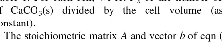
We have investigated a variety of cases, but have selected three test cases which illustrate these interactions. We first describe these cases qualitatively. In the first two cases, under the control of a steady inflow of basic solution, each cell passes from acidic to basic and, consequently, each carbonate species dominates in turn; the second cell follows the first in wave-like fashion. The dominant car-bonate species can be seen in the concentration histories of Fig. 2, for Case 1. Each cell shows periods of relatively slow change of pH within these regimes, separated by short transition intervals in which the pH and the distribution of carbonate species vary rapidly. The Hþ ion concentration starts at 10¹3mol l¹1(i.e. pH 3) in each cell and dissolved H2CO3 is initially the dominant carbonate species.
How-ever, in cell 1, the pH rises to between 5 and 7 in the interval 200, t,600 s and HCO3¹ becomes dominant. This pat-tern occurs in cell 2 for 600,t,1100 s. In cell 1, the pH then takes another rise to pH.10 fort.700 s and CO23¹ dominates at about 10¹4
M and HCO3¹ drops to about
10¹5
M. The same pattern occurs in cell 2 at t . 1300 s. The time scales of these observations are determined by the physical transport, i.e. the volumetric flow rates and cell sizes
Fig. 2. Profiles of Hþ and aqueous carbonate species showing
arbitrarily set to about 1 l. All our concentrations will sub-sequently be given in mol l¹1and all times in seconds.
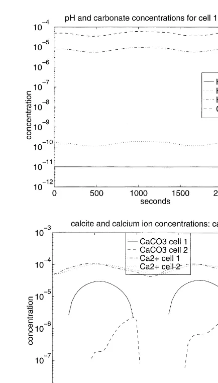
For Case 1 that we just described, the cell solutions remain undersaturated with respect to calcite throughout. Case 2 has essentially the same history for the carbonate species; however, as the CO2¹
3 concentration rises in which
cell, the solution becomes saturated and a period of preci-pitation of solid CaCO3occurs, followed by its dissolution,
in each cell. Fig. 3 shows this episode of precipitation occur-ring for 600,t,1700 s in cell 1 and occurring for 1200,
t,2600 s in cell 2.
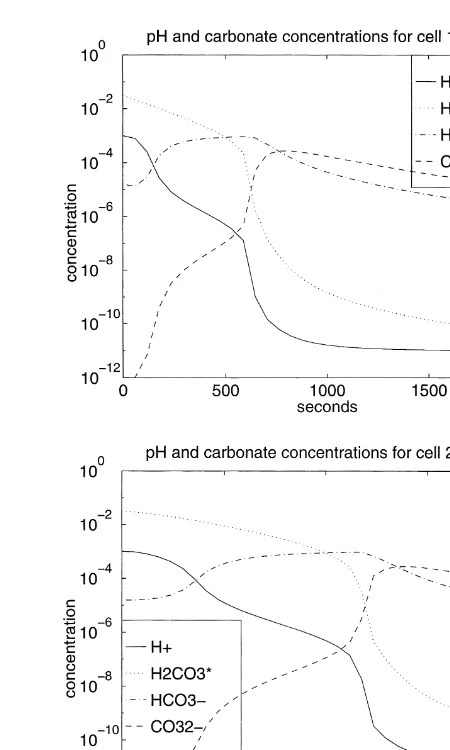
The first two cases illustrate the cells progressing through the transitions in the dominant dissolved carbonate species with and without precipitation. The third case demonstrates changes in the saturation state in a basic solution with no transitions in the dominant carbonate species. The concentra-tion histories for Case 3 are shown in Fig. 4. Initially, there is no calcite in either cell. The inflow of Ca2þis varied so that two episodes of precipitation and complete dissolution occur in each cell at slightly staggered intervals. While this is per-haps not a realistic scenario, it provides a computational con-trol case for distinguishing between the effects of transitions in dominant carbonate species and the effect of dissolution/ precipitation on the methods for solving the implicit time stepping equations.
4.2 Details of the demonstration cases
Cases 1 and 2 are identical in all respects, except for the higher calcium concentrations used to trigger precipitation in Case 2, and the simulation period is longer for Case 2. There are special computational difficulties associated with the computational solution of DAE systems when the initial states do not satisfy the algebraic equations, i.e. the initial simulation state is not in quasi-equilibrium. Since we are demonstrating effects associated with changes in chemical regimes, we avoid initial transient difficulties by spreading the change between the inflow pH and the initial cell pH
over an initial period of 100 s. All concentrations are in units of mol l¹1, as indicated in Section 2. The initial states are the same in Cases 1 and 2; the following values are common to both cells:
• The initial states:
C1,k¼10¹12 CO23¹]
ÿ ,
C3,k¼10¹3 Hþ
ÿ ,
C4,k¼10
¹11 OH¹
½ ÿ ð Þ,
C5,k¼1:585310¹5 HCO3¹
ÿ ,
C6,k¼3:165310
¹2
H2CO3
ÿ ,
Pk¼0; i:e:no precipitate in either cell:
• Volumetric flow rates: v0¼0.008 l s¹1,
v1¼0.0085 l s¹1
.
• Constant inflow concentrations:C1,in¼10¹5, C5,in¼5 310¹7
,C6,in¼53 10¹9
.
• Variable inflow concentrations:
C3,in(t)¼(1¹t=100)10
¹3þ(
t=100)10¹11
fort,100 ¼10¹11 for t.100:
Fig. 3. Concentration histories of Ca2þ and CaCO
3 (solid
pre-cipitate): Case 2.
Note:Tin ¼ACin.
• Maximum time step parameter qmax ¼ 0.5, cell
sizesh1¼1,h2¼2 l.
The differences between Cases 1 and 2 are that the simu-lated time is longer (2000 and 2800 s, respectively), and the initial and inflow concentrations of Ca2þ
areC2,k¼10¹5
in Case 1 andC2,k¼5310¹5
in Case 2. Because no precipita-tion occurs in Case 1,C2,k(t) values are constant; the history
ofC2,k(t) for Case 2 is shown in Fig. 3.
For Case 3, the cells each experience two episodes of precipitate forming and then dissolution, as shown in Fig. 4.
• Initial states are the same in both cells and are:
C1,k¼5310
¹5, C
2,k¼5310
¹5, C 3,k¼10
¹11,
C4,k¼10¹3, C5,k¼8:0310¹6,
C6,k¼1:7310¹10, Pk¼0:
• Volumetric flow rates:v0¼0.005,
v1¼0.0052 l s¹1
.
• Constant inflow concentrations:
C1,in¼5310¹5, C3,in¼10¹11, C4,in¼10¹3,
C5,in¼8:0310¹6, C6,k¼1:7310
¹10:
• Variable inflow concentrations:
C2,in(t)¼max[0, 10¹5(5þ15sin(2pt=1200))]: • Final time¼2400 s; maximum time step parameter
qmax¼13; cell sizesh1¼2,h2¼0.5 l.
4.3 Observations about computations with the standard Newton method
We first discuss the performance of the global linearization approach and the SIA approach when both use the standard form of Newton’s method.
4.3.1 Case 1
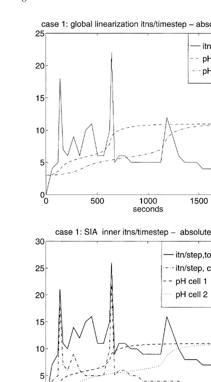
A basic observation for this case is that both methods experience difficulty during the intervals of transition between dominant carbonate species. Computational diffi-culty, or cost, at a certain time takes the form of an increase in the number of iterations required to take a time step, including the possibility that one or more reductions of dt
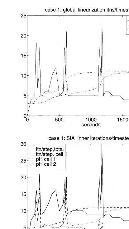
may be required in order to make a successful step. This can be seen in the plots of Fig. 5, in which the solid line shows the iterations/step at each time. Global linearization is shown at the top and the inner SIA iterations, totaled for both cells, at the bottom. The pH history for cell 1 (dashed) and cell 2 (dashed-dotted) are superimposed on these plots to reference the carbonate transitions. The peaking of the iterations/step at the transitions is clearly apparent for both methods. In general terms, it represents the response of the methods to the stiffness of the equations that occurs at the transitions. These plots show the total number of iterations required to make the time step;
more than 12 iterations per step are accompanied by step size reduction.
This figure illustrates how a source of computational dif-ficulty is localized in time, i.e. at the relatively short times of the carbonate transitions. However, in this history the tran-sitions occur in one cell at a time, i.e. they are also localized in space. One of the benefits sought from using SIA is that it can reduce costs relative to global linearization by localiz-ing the computational difficulties in space. This effect can be seen in the lower plot of Fig. 5. The dashed-dotted line in this plot shows the contribution to the total iterations/step from the iterations occurring in the first cell. The transitions for the first cell occur att¼200 and 600 s, and the peaks of the iterations/step in the first cell are clearly the dominant contribution to the total iterations/step at that time. Simi-larly, the transitions in the second cell occur att¼400 and 1200 s, but relatively low numbers of iterations/step occur in the first cell at those times.
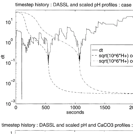
The sharp peaking of the iterations per step profiles at the transition times is associated with time step reductions at those times, which is an extreme form of computational difficulty, or cost. Both approaches experience time step reductions to essentially the same degree. At the top of
Fig. 7, the time step history for global linearization is shown, again superimposed on a scaled pH history for reference.
Since the carbonate transitions are the only dynamical features of Case 1, it is not surprising that the computational difficulty is concentrated at these times. In particular, the absence of calcite allows SIA to terminate its outer iteration in two steps, as discussed in Section 3, so that Case 1 is somewhat atypical for SIA.
4.3.2 Case 2: the impact of dissolution/precipitation
In Case 2, we add a dynamic dissolution/precipitation pro-cess, as discussed above. The histories of the carbonate species are essentially the same as Case 1. However, as a result of the increased inflow of Ca2þ
, the calcite concentra-tion in cell 1 is zero until aboutt¼600 s, at which time it appears in Fig. 3, as the solid line. Precipitation is followed by dissolution, as the CO23¹ drops and the calcite vanishes from cell 1 at about 1650 s. The calcite history in cell 2 is similar; it first appears at aboutt¼1200 s and vanishes at aboutt¼2500 s.
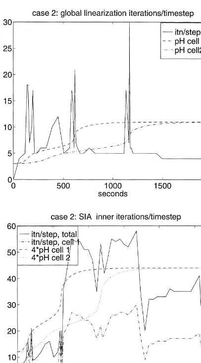
If we turn to the plots of iterations per step for this case, shown in Fig. 6, we can see that global linearization
performs essentially the same as for Case 1.2 However, the performance for SIA is substantially affected by the appearance of the precipitate. (Note the changes in scale, including the scaling of the pH reference curves from Fig. 5.) The peaking of the histories associated with the carbonate transitions are still in evidence. However, these peaks are dominated by several plateaus associated with the presence of calcite in the cells. These ‘solution difficulty’ plateaus are also somewhat localized in space, as the drop of the plateau after the disappearance of calcite from cell 1 indicates. Note that the transitions between the undersaturated and satu-rated states do not appear to cause any computational diffi-culty for either method, which seems counter to other experiences. The time step reductions for this case are iden-tical to Case 1, so they are clearly triggered by the carbonate transitions.
We can gain further insight into the coupled iterations of SIA for Case 2 by looking at the plots at the bottom of Fig. 7, which show the number of outer iterations at each time step
Fig. 6.Iterations per step and scaled pH histories: Case 2.
Fig. 7. (Left) Time step size: Case 1. (Right) Iterations of SIA:
Case 2.
2
in the upper graph and the ratio of inner to outer iterations at each time step in the lower one. The effects of the stiffness associated with the carbonate transitions on the inner itera-tions are clearly subordinate to the outer iteration in the presence of precipitate.
4.3.3 Case 3: confirming these observations
In Case 3, CO23þ is the dominant carbonate species, and two episodes of precipitate appearing and disappearing occur in each cell. The global linearization proceeds with little variation in the number of iterations per step, as would be anticipated from the previous observations. Neither method exhibits any time step reductions. The profile of total inner iterations per time step for SIA is shown at the top in Fig. 8; it shows the same pattern of dependence on the presence of calcite as was observed in Case 2. The profiles of the outer iterations and inner iteration (outer iteration) are at the bottom of this same figure, and show the same features as the graph on the left of Fig. 7.
The outer iteration is global in the sense that the presence of precipitate in any one cell triggers it globally. However, Figs 7 and 8 appear to show some differentiation in the total
numbers of outer iterations required, depending on whether the calcite is present in cell 1 only, cell 2 only, or both. Perhaps this is due to the simple transport coupling of the mixing cell model; in any case, it is a subtle effect in these results.
4.4 Modifying Newton’s method to maintain positive iterates
There are two motivations for using modifications of Newton’s method that arise in the context of this study. One is more efficient iteration during chemical reaction stiffness, as exhibited by the carbonate transitions. The other motivation is that reactive transport models that are more complex than we have used in these demonstrations commonly require the iterates for concentration variables to be positive, or at least non-negative (e.g., Forsyth6 or Meintjes and Morgan11). The standard Newton method as reported above does not ensure this; indeed, negative con-centrations occur frequently during the iterations of both the global linearization and the second stage of SIA.
One of the strengths of the standard Newton method is its
convergence speed after its iteration sequence enters quad-ratic convergence mode. To obtain six significant digits, once quadratic convergence starts, would seldom take more than three iterations. The above iterations/time step profiles show that Newton’s method is operating in quad-ratic convergence mode most of the time during these simu-lations. However, during the carbonate transition periods of Cases 1 and 2, Newton’s method in both global linearization and SIA suddenly requires 10–30 iterations/time step. At least conceptually, most of these iterations are spent search-ing solution space for an entry into a region of quadratic convergence to some solution of the equations. During this phase, the full linearization used by Newton’s method can lead to large updates, and consequently negative iterates. In this demonstration, these difficulties are infrequent and only contribute a small amount to the total amount of computa-tion; however, in a finite element or finite volume simula-tion, these transitions can occur most of the time in one or more locations.
There are several remedies that have been employed for this. One of them, which we have already introduced, is to reduceDt. This has the effect of making the solution at the previous time step a better estimate for the solution at the
current time. Time step reduction is a necessary capability for implicit time stepping to handle failures of the iteration methods to solve the implicit equations. However, it is a rela-tively expensive procedure. Another possible source of improvement would be to modify the functions that appear in the model equations for non-physical values of their argu-ments. A simple example of this has been shown in the defini-tion ofg4in eqn (17). The basic idea is to make the model
equations tolerant of non-physical arguments, but not admit any solutions with non-physical values. We experimented with this approach, but found that, at least for the relatively simple modifications that we tried, this was not effective.
A common modification of Newton’s method is to incor-porate line searching to ensure that successive iterates reduces the residual of the equations to be solved. There is a large literature on line searching techniques primarily associated with optimization; a discussion oriented to chemical reaction equilibria computations is presented in Smith and Missen.16 We experimented with the method described on pp. 114 and 115 of this reference; it updates the current iterate by a fraction of the Newton correction, when the equation’s residual has a minimum on the line segment between consecutive Newton iterates. The tech-nique was activated using several different criteria. In none of these instances did it improve on the standard Newton method’s cumulative performance for any of the demonstration simulation cases, and under some criteria it performed significantly worse. We believe that a qualitative explanation for this lies in a mismatch between the basic tactic of line searching and the source of computational difficulty for these dynamic simulation computations. Line searching attempts to control the update of an iteration by sensing the behavior of the equation’s residual. For Newton’s method, the update and the residual are coupled through the Jacobian matrix of the system of equations. The episodes of difficulty for Newton’s method have been shown in Figs 5 and 6 to be connected to the periods of rapid change in the concentrations. These rapid changes are characterized in several equivalent ways, short time scales for the linearized dynamic equations, stiffness for iteration methods and ill-conditioned Jacobian matrices. The implication of this last characterization is that the Newton correction is poorly determined by the equation residual. We believe this mitigates against the usefulness of line searching, which seeks to improve performance by controlling the residual, rather than the update directly.
An approach that we found more successful was to modify the updates of Newton’s method. The primary moti-vation for these modifications is to prevent non-positive iterates, but they have the complimentary benefit of limiting the size to the Newton update when it is not in quadratic convergence mode as well. Meintjes and Morgan11 pro-posed using the absolute value of the updated iterate, i.e.
Cjnþ1,k¼lC nþ1,k¹1
j þupdatejl (30)
for chemical equilibrium computations. We will refer to this as the absolute update technique. An alternative tactic
is to limit the downwards change in the iterates, i.e. for a downward change limited to the 5% level:
Cjnþ1,k¼max Cjnþ1,k¹1þupdatej, 0:05C nþ1,k¹1
j
:
(31)
We will refer to this as an LDC at 0.05 update; we also demonstrate the LDC at 0.0001 update below.
4.4.1 Case studies reviewed for positive iterates
The use of the absolute update and LDC update modi-fications produced positive iterates and reduced the peak numbers of iterations per time step, and the time size reduc-tions, taken by both global linearization and SIA. Fig. 9 shows this effect for Case 1.
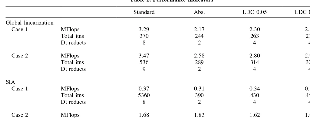
A summary of performance data using the standard Newton iteration and the modified updates versions is given in Table 2 for both iteration methods. Note that the data marked ‘Total itns’ in these tables is not comparable for global linearization and SIA, since it is the total number of global Newton iterations in the former context, but the total number of single cell inner iterations in the latter context. The absolute update technique performed marginally better in these tests, but basically the improvement is essentially the same for all three reported results.
In Case 2, as in Case 1, improvements in iteration effi-ciencies from the update modifications are observed during the stiffness periods associated with the carbonate transi-tions. However, after these transitions, fort. 1200 s, the standard Newton method, both for global linearizatiion and for SIA, is always operating in essential quadratic conver-gence mode with non-negative iterates. Global linearization is unaffected by the dissolution/precipitation reaction, so the efficiency improvement associated with the update modifi-cation is about the same as for Case 1, diluted somewhat by the longer simulation period of Case 2. As we have noted
above, the predominant factor in the amount of computation for SIA in the presence of precipitate is the number of outer iterations per time step. Hence, for SIA the efficiency improvement from the modified updates are minor in Case 2. In Case 3, the standard Newton method always operated with non-negative iterates, so update modifications had no effect on performance for this case.
5 CONCLUSIONS
The tests reported in the previous section and other testing on this model problem suggest the following qualitative conclusions.
• The computational difficulty for Newton’s method exhibited during the transitions in dominant carbo-nate species indicates a basic stiffness of the model equations. Since this stiffness can be localized in space, its effect on Newton’s method in SIA can be expected to be localized to the inner iterations of the affected spatial regions, and possibly adjacent locations.
• When SIA requires outer iterations, the conver-gence of the outer iterations appears to be the limit-ing factor in the computational efficiency of the method.
• The formulation of the saturated/undersaturated cal-cite equilibrium condition as a single algebraic equation, eqn (18), is computationally effective.
• The use of the non-negative update modification of Newton’s method not only ensures non-negative concentrations during the iterations, but can also improve computational efficiency.
None of these conclusions is particularly radical, although we think it is useful to have demonstrated their
Table 2. Performance indicators
Standard Abs. LDC 0.05 LDC 0.0001
Global linearization
Case 1 MFlops 3.29 2.17 2.30 2.47
Total itns 370 244 263 277
Dt reducts 8 2 4 4
Case 2 MFlops 3.47 2.58 2.80 2.91
Total itns 536 289 314 325
Dt reducts 9 2 4 4
SIA
Case 1 MFlops 0.37 0.31 0.34 0.36
Total itns 5360 390 430 447
Dt reducts 8 2 4 4
Case 2 MFlops 1.68 1.83 1.62 1.64
Total itns 1844 1986 1757 1785
Dt reducts 7 2 4 4
role in the similarities and differences between global line-arization and SIA. This micro-model has allowed a detailed look at the two methods. Although it is too small for prac-tical comparisons of computing resource usage, we have included in Table 2 the count of floating point operations required for each computation of Cases 1 and 2. Case 1 is atypically favorable to SIA, since exactly two outer itera-tions are used; however, Case 2 shows that SIA takes between 1/2 and 2/3 of the amount of arithmetic that global linear-ization takes, even on these small computations.
It appears to us that the formulation of the dissolution/ precipitation equilibrium conditions as the single algebraic equation, eqn (18), can be directly extended to multiple dissolution/precipitation reactions.
We believe that these conclusions will retain much of their validity, at least qualitatively, in larger model compu-tations with more sophisticated numerical methods. Here, we look briefly at the performance of the public domain DAE code DASSL for our demonstration cases. DASSL is based on global linearization for variable order implicit time stepping (see Brenanet al.3for further details). In Fig. 10, we show the time step profiles of DASSL applied to Cases 1 and 2.
The volatility of the step size profile for DASSL is clear; note that the vertical axis for the plot uses a log scale. DASSL uses time step modification more aggressively than the conservative strategy outlined in Section 3 for our computations. The DASSL strategy incorporates accu-racy control as well as handling non-convergence of the process for solving the implicit time stepping equations. This process is a refinement of Newton’s method, and non-convergence is assumed after much fewer iterations than the maximum of 12 we have used. Despite these dif-ferences, the large reductions in step size at times of transi-tion between dominant carbonate species are clearly evident in the DASSL time step profile shown on the left of Fig. 10. The fact that the transitions between undersaturated and saturated states did not cause any noticeable difficulty for Newton’s method in either the global linearization or the inner SIA iterations was unexpected. The very dramatic effect on DASSL of the appearance of precipitate in the cells can be seen in the time step profile on the right of Fig. 10. The concentration of precipitate in cell 1 is shown with a curve of long-short dashes on this graph. The reduc-tions inDtassociated with the carbonate transitions that we noted for Case 1 (on the left) can still be seen. However, very shortly after these the step size plunges to 10¹6
with the appearance of calcite in first cell 1, then cell 2 (see Fig. 3). The difficulties that occur for DASSL when the functions of the DAE system are not smooth have been discussed in Ref. 3, Section 5.3.3. In particular, an extension of this code is discussed which is designed to support switching between versions of the system functions. Engesgaard and Kipp5 reported sharp peaks to about 60 SIA iterations/time step at the time that a moving dissolution front empties a new finite volume cell, for their formulation of the model equa-tions and SIA. However, this peak quickly dies back to a
small number of iterates, while the cells all remain in the same saturation state.
ACKNOWLEDGEMENTS
This research was supported by the Groundwater Research Center and the Information Technology Research Center, both of which are part of the Ontario Centers of Excellence program, and also by the Natural Science and Engineering Research Council of Canada.
REFERENCES
1. Barry, D. A., Bajracharya, K. and Miller, C. T. Alternative split-operator approach for solving chemical reaction/ groundwater transport models. Adv. Water Resour., 1996, 19,261–275.
2. Bethke, C. M., Geochemical Reaction Modeling. Oxford University Press, Oxford, 1996.
3. Brenan, K. E., Campbell, S. L. and Petzold, L. R.,Numerical Solution of Initial-Value Problems in Differential-Algebraic Equations. North-Holland, 1989.
4. Cederberg, G. A., Street, R. L. and Leckie, J. O. A ground-water mass transport and equilibrium chemistry model for multicomponent systems. Water Resour. Res., 1985, 19, 1095–1104.
5. Engesgaard, P. and Kipp, K. L. A geochemical model for redox-controlled movement of mineral fronts in ground water flow systems: a case of nitrate removal by oxidation of pyrite.Water Resour. Res., 1992,28,2829–2843. 6. Forsyth, P. A. A positivity preserving method for simulation
of steam injection for NAPL site remediation. Adv. Water Resour., 1993,16,351–370.
7. Forsyth, P. A., Wu, Y. S. and Pruess, K. Robust numerical methods for saturated–unsaturated flow with dry initial con-ditions in heterogeneous media.Adv. Water Resour., 1995, 18,25–38.
8. Herzer, J. and Kinzelbach, W. Coupling of transport and chemical processes in numerical transport models. Geo-derma, 1989,44,115–127.
9. Lichtner, P. C., Steefel, C. I. and Oelkers, E. H., ed.Reactive Transport in Porous Media,Reviews in Mineralogy, Vol. 34. Mineralogical Society of America, 1996.
10. Marzal, P., Seco, A., Ferrer, J. and Gabaldon, C. Modeling multiple reactive solute transport with adsorption under equi-librium and non-equiequi-librium conditions.Adv. Water Resour., 1994,17,363–374.
11. Meintjes, K. and Morgan, A. Chemical equilibrium systems as numerical test problems. ACM Trans. Math. Software, 1990,16,143–151.
12. Morel, F. and Morgan, J. A numerical method for computing equilibria in aqueous chemical systems.Environ. Sci. Tech-nol., 1972,20,58–67.
13. Rubin, J. Transport of reacting solutes in porous media: rela-tion between mathematical nature of problem formularela-tion and chemical nature of reactions. Water Resour. Res., 1983,19(5), 1231–1252.
16. Smith, W. R. and Missen, R. W.,Chemical Reaction Equili-brium Analysis: Theory and Algorithms. John Wiley, New York, 1982.
17. Steefel, C. I. and MacQuarrie, K. T. B.,Reactive Transport in Porous Media,Reviews in Mineralogy, Vol. 34. Mineralogi-cal Society of America, 1996, pp. 83–129.
18. Stumm, W., and Morgan, J. J.,Aquatic Chemistry: Chemical Equilibria and Rates in Natural Waters, 3rd edn. John Wiley, New York, 1996.
19. Yeh, G. T. and Tripathi, V. S. A critical evaluation of recent developments in hydrogeochemical transport models of reac-tive multichemical components.Water Resour. Res., 1989, 25(1), 93–108.
20. Yeh, G. T. and Tripathi, V. S. A model for simulating trans-port of reactive multispecies components: model develop-ment and demonstration.Water Resour. Res., 1991,27(12), 3075–3094.
21. Zysset, A., Stauffer, F. and Dracos, T. Modelling of chemi-cally reactive groundwater transport. Water Resour. Res., 1994,30(7), 2217–2228
APPENDIX A EXISTENCE OF A PHYSICALLY MEANINGFUL SOLUTION OF THE IMPLICIT TIME STEPPING EQUATIONS
We present here the mathematics to support the claims that there always exists a physically meaning solution of the second stage SIA equations, eqns (27)–(29), and similarly for the uncoupled implicit time stepping equations, eqns (19)–(22), for any size ofDt.
If we uncouple the mixing cells by settingv1(t)¼v0(t), so that v2¼ 0, V1,0 ¼v0(t)/h1andV1,1¼ ¹v0(t)/h1, we can
introduce the single flow parameterq¼Dtv0(tnþ1)/h1. If we
then drop the cell index,k, from variables Ti,k,Ci,kandPk, we can write eqns (19) and (20) as: the first cell. If we subtract eqn (A1) from eqn (A2), we get, settingqi¼T(
This is the same form as occurs in the second stage SIA equation, eqn (26); in this latter case, we can identify the superscript (nþ1) with (nþ1,j),qiwithTi(nþ1,j)andq¼0. Dropping all super- and subscripts except the species designators, we can write the form of the equations as:
C1þC5þC6¼(q1¹P)=(1þq) (A4)
We first introduce parametersrandsfor unknown concen-trationsC3andP, respectively, and show that we can solve
eqns (A4), (A7), (A8) and (A9) for C1, C4,C5and C6in terms of (r,s). In fact, it is immediate that
C4(r,s)¼K3=r; C5(r,s)¼C1(r,s)r=K1;
C6(r,s)¼C1(r,s)r2=K2: ðA11Þ
Substituting eqn (A11) into eqn (A4), we determineC1(r,s) as
C1(r,s)(1þr=K1þr2=K2)¼(q1¹s)=(1þq): (A12)
We can now use eqn (A6) and C3 ¼ r to determine a relation between (r,s) such that solutions Cj for j ¼ 1 to 6 of eqns (A4) to (A9) can be parameterized by the single parameter,s. Eqn (A6) will be satisfied withrdependent on
s.0 if we can solve (A9) parameterized by s.
We now analyze eqn (A10) to determine a non-negative values* ofssuch that
g4(C1(sp), C2(sp), sp)¼0, (A16)
thenCj(s*) andP(s*) will provide a solution to eqns (A3) and (A10). From eqns (A12) and (A5), we can see that
C1(0) . 0 and C2(0) . 0. Looking at the definition (17) of g4, we can see that the analysis breaks down into two cases based on whetherC1(0)C2(0)# Kspor not:
case (a):C1(0)C2(0)#Ksp, so thatg4(C1(0),C2(0), 0)¼0.
Thus,s*¼0 solves eqn (A16);
case (b):C1(0)C2(0).Ksp, so thatg4(C1(0),C2(0), 0) , 0, which needs further discussion.
In case (b), we will show that there is a positive value ofs
for which eqn (A16) holds by examining the path of (C1(s),
C2(s)) assincreases froms¼0. Since, from eqn (A5),C2(0) ¼q2/(1þq).0, we can conclude thatC1(0).0. Consider
is the hyperbolaC1C2¼Kspin the first quadrant. The con-ditions of case (b) are that (C1(0), C2(0)) lies in the first quadrant above this hyperbola. We now follow (C1(s),
C2(s)) as sincreases. C2(s) ¼(q2 ¹s)/(1þq) decreases linearly assincreases. From eqn (A12),C1(s)¼(q1¹s)/ [(1þq)((1þr(s)/K1þr(s)2/K2)], so that as long asq1¹s
. 0, we have C1(s) , (q1 ¹ s)/(1 þ q) and C1(s) also
decreases assincreases. Hence, there must be a first positive value of s, which we identify as s*, such that (C1(s*), (C2(s*)) crosses the calcite equilibrium curve, and in doing so solves eqn (A16).
Hence, in any event, there is at least one non-negative solution of eqn (A16) and we can note that, from the defini-tion (17) ofg4, there are no solutions of eqn (A16) withs*,0. We note thatC1(s*),C2(s*) are positive (includings*¼0.) FromC3(s*)¼r(s*)¼r(s*) and from the parametrizations (A11), we can see that Ck(s*) . 0 for k ¼ 1 to 6, excluding k ¼ 4. We note that C4 is not required to be positive to be physically meaningful.
APPENDIX B IDENTIFICATION OF MIXING CELL MODEL WITH A FINITE VOLUME METHOD FOR SIMPLE ADVECTIVE–DIFFUSIVE TRANSPORT
Consider Fig. 1 interpreted as a two finite volume cell approximation for advective–diffusive transport ofNS dis-solved species. The cells are aligned with thexcoordinate axis and are normalized to have unit cross-section and lengthh. The cells have a common interface atx0¼0 and boundary interfaces atx¹1¼ ¹h,x1¼ þh. Using the
nota-tion of Appendix 2, we let NS vectors C1 and C2 be the concentrations of dissolved species in cells 1 and 2. The total component concentrations are Tk ¼ ACk using the
stoichiometric matrix of eqn (14). The connecting ‘pipes’ across these interfaces are conceptually replaced by finite volume transport mechanisms. We identify the upwinded finite volume flux (mol m¹2
s¹1
) of total component con-centrations acrossx0as:
f0(t)¼ ¹D(AC2¹AC1)=hþUAC1,
whereDis a scalar diffusion coefficient and Uis a scalar advection coefficient, or transport rate.
We identify f¹1 ¼UTin(t) as a prescribed flux of total
concentrations into cell 1 through the boundary interface atx¹1andf1¼UAC2as the condition on the flux through
the boundary interface atx1.
The conservation equations for the total concentrations,
Ti, in finite volume celliare:
hdT1
dt ¼f¹1¹f0 (B1)
¼UTin(t)¹(D=hþU)AC1(D=h)AC2,
hdT2
dt ¼f0¹f1¼(D=hþU)AC1:
We can now identify eqn (B1) with the mixing cell equa-tion, eqn (3), by identifying
v0(t)¼U andv1(t)¼D=hþU:
Note that this identification imposes on the mixing cell velocities the requirement that v1(t) ¹ v0(t) . 0, since
v1(t) ¹ v0(t) is identified with D/h; this is requirement (1). Hence, the choice of v0 ¼ 0.008 and v1 ¼ 0.0085 l s¹1 in demonstration Case 1 could be regarded as an advection-dominated transport (U ¼ 0.008, D/h ¼ 0.0005 l m¹2
s¹1