i
Lecture Notes on Optimization
Contents
1 INTRODUCTION 1
2 OPTIMIZATION OVER AN OPEN SET 7
3 Optimization with equality constraints 15
4 Linear Programming 27
5 Nonlinear Programming 49
6 Discrete-time optimal control 75
7 Continuous-time linear optimal control 83
8 Coninuous-time optimal control 95
9 Dynamic programing 121
PREFACE to this edition
Notes on Optimizationwas published in 1971 as part of the Van Nostrand Reinhold Notes on Sys-tem Sciences, edited by George L. Turin. Our aim was to publish short, accessible treatments of graduate-level material in inexpensive books (the price of a book in the series was about five dol-lars). The effort was successful for several years. Van Nostrand Reinhold was then purchased by a conglomerate which cancelled Notes on System Sciences because it was not sufficiently profitable. Books have since become expensive. However, the World Wide Web has again made it possible to publish cheaply.
Notes on Optimization has been out of print for 20 years. However, several people have been using it as a text or as a reference in a course. They have urged me to re-publish it. The idea of making it freely available over the Web was attractive because it reaffirmed the original aim. The only obstacle was to retype the manuscript in LaTex. I thank Kate Klohe for doing just that.
I would appreciate knowing if you find any mistakes in the book, or if you have suggestions for (small) changes that would improve it.
Berkeley, California P.P. Varaiya September, 1998
PREFACE
TheseNoteswere developed for a ten-week course I have taught for the past three years to first-year graduate students of the University of California at Berkeley. My objective has been to present, in a compact and unified manner, themainconcepts and techniques of mathematical programming and optimal control to students having diverse technical backgrounds. A reasonable knowledge of advanced calculus (up to the Implicit Function Theorem), linear algebra (linear independence, basis, matrix inverse), and linear differential equations (transition matrix, adjoint solution) is sufficient for the reader to follow theNotes.
The treatment of the topics presented here is deep. Although the coverage is not encyclopedic, an understanding of this material should enable the reader to follow much of the recent technical literature on nonlinear programming, (deterministic) optimal control, and mathematical economics. The examples and exercises given in the text form an integral part of theNotesand most readers will need to attend to them before continuing further. To facilitate the use of theseNotesas a textbook, I have incurred the cost of some repetition in order to make almost all chapters self-contained. However, Chapter V must be read before Chapter VI, and Chapter VII before Chapter VIII.
The selection of topics, as well as their presentation, has been influenced by many of my students and colleagues, who have read and criticized earlier drafts. I would especially like to acknowledge the help of Professors M. Athans, A. Cohen, C.A. Desoer, J-P. Jacob, E. Polak, and Mr. M. Ripper. I also want to thank Mrs. Billie Vrtiak for her marvelous typing in spite of starting from a not terribly legible handwritten manuscript. Finally, I want to thank Professor G.L. Turin for his encouraging and patient editorship.
Berkeley, California P.P. Varaiya November, 1971
Chapter 1
INTRODUCTION
In this chapter, we present our model of the optimal making problem, illustrate decision-making situations by a few examples, and briefly introduce two more general models which we cannot discuss further in theseNotes.
1.1
The Optimal Decision Problem
TheseNotesshow how to arrive at an optimal decision assuming that complete information is given. The phrasecomplete information is givenmeans that the following requirements are met:
1. The set of all permissible decisions is known, and 2. The cost of each decision is known.
When these conditions are satisfied, the decisions can be ranked according to whether they incur greater or lesser cost. Anoptimal decisionis then any decision which incurs the least cost among the set of permissible decisions.
In order to model a decision-making situation in mathematical terms, certain further requirements must be satisfied, namely,
1. The set of all decisions can be adequately represented as a subset of a vector space with each vector representing a decision, and
2. The cost corresponding to these decisions is given by a real-valued function. Some illustrations will help.
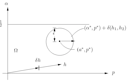
Example 1: The Pot Company (Potco) manufacturers a smoking blend called Acapulco Gold. The blend is made up of tobacco and mary-john leaves. For legal reasons the fractionαof mary-john in the mixture must satisfy0< α < 12. From extensive market research Potco has determined their expected volume of sales as a function ofαand the selling pricep. Furthermore, tobacco can be purchased at a fixed price, whereas the cost of mary-john is a function of the amount purchased. If Potco wants to maximize its profits, how much mary-john and tobacco should it purchase, and what pricepshould it set?
Example 2: Tough University provides “quality” education to undergraduate and graduate stu-dents. In an agreement signed with Tough’s undergraduates and graduates (TUGs), “quality” is
defined as follows: every year, eachu(undergraduate) must take eight courses, one of which is a seminar and the rest of which are lecture courses, whereas eachg(graduate) must take two seminars and five lecture courses. A seminar cannot have more than 20 students and a lecture course cannot have more than 40 students. The University has a faculty of 1000. The Weary Old Radicals (WORs) have a contract with the University which stipulates that every junior faculty member (there are 750 of these) shall be required to teach six lecture courses and two seminars each year, whereas every senior faculty member (there are 250 of these) shall teach three lecture courses and three seminars each year. The Regents of Touch rate Tough’s President atαpoints peruandβ points perg “pro-cessed” by the University. Subject to the agreements with the TUGs and WORs how manyu’s and
g’s should the President admit to maximize his rating?
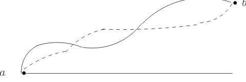
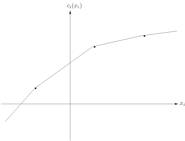
Example 3: (See Figure1.1.) An engineer is asked to construct a road (broken line) connection point a to pointb. The current profile of the ground is given by the solid line. The only requirement is that the final road should not have a slope exceeding 0.001. If it costs $cper cubic foot to excavate or fill the ground, how should he design the road to meet the specifications at minimum cost?
Example 4: Mr. Shell is the manager of an economy which produces one output, wine. There are two factors of production, capital and labor. IfK(t)andL(t)respectively are the capital stock used and the labor employed at timet, then the rate of output of wineW(t)at time is given by the production function
W(t) = F(K(t), L(t))
As Manager, Mr. Shell allocates some of the output rateW(t)to the consumption rateC(t), and the remainderI(t)to investment in capital goods. (Obviously,W,C,I, andKare being measured in a common currency.) Thus,W(t) = C(t) +I(t) = (1−s(t))W(t)wheres(t) =I(t)/W(t)
.
.
a
b
Figure 1.1: Admissable set of example.
∈[0,1]is the fraction of output which is saved and invested. Suppose that the capital stock decays exponentially with time at a rate δ > 0, so that the net rate of growth of capital is given by the following equation:
˙
K(t) = d
dtK(t) (1.1)
= −δK(t) +s(t)W(t)
= −δK(t) +s(t)F(K(t), L(t)).
1.1. THE OPTIMAL DECISION PROBLEM 3
˙
L(t) = βL(t).
(1.2) Suppose that the production function F exhibits constant returns to scale, i.e., F(λK, λL) =
λF(K, L) for all λ > 0. If we define the relevant variable in terms of per capita of labor, w =
W/L, c=C/L, k =K/l, and if we letf(k) =F(k, l), then we see thatF(K, L)−LF(K/L,1) =
Lf(k), whence the consumption per capita of labor becomesc(t) = (l−s(t))f(k(t)). Using these definitions and equations (1.1) and (1.2) it is easy to see thatK(t)satisfies the differential equation (1.3).
˙
k(t) = s(t)f(k(t))−µk(t)
(1.3) whereµ= (δ+β). The first term of the right-hand side in (3) is the increase in the capital-to-labor ratio due to investment whereas the second terms is the decrease due to depreciation and increase in the labor force.
Suppose there is a planning horizon timeT, and at time0Mr. Shell starts with capital-to-labor ratioko. If “welfare” over the planning period[0, T]is identified with total consumption
RT
0 c(t)dt, what should Mr. Shell’s savings policys(t), 0 ≤ t ≤ T, be so as to maximize welfare? What savings policy maximizes welfare subject to the additional restriction that the capital-to-labor ratio at timeTshould be at leastkT? If future consumption is discounted at rateα >0and if time horizon is∞, the welfare function becomesR∞
0 e−αt c(t)dt. What is the optimum policy corresponding to this criterion?
These examples illustrate the kinds of decision-making problems which can be formulated math-ematically so as to be amenable to solutions by the theory presented in theseNotes. We must always remember that a mathematical formulation is inevitably an abstraction and the gain in precision may have occurred at a great loss of realism. For instance, Example 2 is caricature (see also a faintly re-lated but more more elaborate formulation in Bruno [1970]), whereas Example 4 is light-years away from reality. In the latter case, the value of the mathematical exercise is greater the more insensitive are the optimum savings policies with respect to the simplifying assumptions of the mathematical model. (In connection with this example and related models see the critique by Koopmans [1967].) In the examples above, the set of permissible decisions is represented by the set of all points in some vector space which satisfy certain constraints. Thus, in the first example, a permissible decision is any two-dimensional vector (α, p) satisfying the constraints 0 < α < 12 and 0 < p. In the second example, any vector (u, g) with u ≥ 0, g ≥ 0, constrained by the number of faculty and the agreements with the TUGs and WORs is a permissible decision. In the last example, a permissible decision is any real-valued function s(t), 0 ≤ t ≤ T, constrained by
At this point, it is important to realize that the distinction between the function which is to be optimized and the functions which describe the constraints, although convenient for presenting the mathematical theory, may be quite artificial in practice. For instance, suppose we have to choose the durations of various traffic lights in a section of a city so as to achieve optimum traffic flow. Let us suppose that we know the transportation needs of all the people in this section. Before we can begin to suggest a design, we need a criterion to determine what is meant by “optimum traffic flow.” More abstractly, we need a criterion by which we can compare different decisions, which in this case are different patterns of traffic-light durations. One way of doing this is to assign as cost to each decision the total amount of time taken to make all the trips within this section. An alternative and equally plausible goal may be to minimize the maximum waiting time (that is the total time spent at stop lights) in each trip. Now it may happen that these two objective functions may be inconsistent in the sense that they may give rise to different orderings of the permissible decisions. Indeed, it may be the case that the optimum decision according to the first criterion may be lead to very long waiting times for a few trips, so that this decision is far from optimum according to the second criterion. We can then redefine the problem as minimizing the first cost function (total time for trips) subject to the constraint that the waiting time for any trip is less than some reasonable bound (say one minute). In this way, the second goal (minimum waiting time) has been modified and reintroduced as a constraint. This interchangeability of goal and constraints also appears at a deeper level in much of the mathematical theory. We will see that in most of the results the objective function and the functions describing the constraints are treated in the same manner.
1.2
Some Other Models of Decision Problems
Our model of a single decision-maker with complete information can be generalized along two very important directions. In the first place, the hypothesis of complete information can be relaxed by allowing that decision-making occurs in an uncertain environment. In the second place, we can replace the single decision-maker by a group of two or more agents whose collective decision determines the outcome. Since we cannot study these more general models in these Notes, we merely point out here some situations where such models arise naturally and give some references.
1.2.1 Optimization under uncertainty.
A person wants to invest $1,000 in the stock market. He wants to maximize his capital gains, and at the same time minimize the risk of losing his money. The two objectives are incompatible, since the stock which is likely to have higher gains is also likely to involve greater risk. The situation is different from our previous examples in that the outcome (future stock prices) is uncertain. It is customary to model this uncertainty stochastically. Thus, the investor may assign probability 0.5 to the event that the price of shares in Glamor company increases by $100, probability 0.25 that the price is unchanged, and probability 0.25 that it drops by $100. A similar model is made for all the other stocks that the investor is willing to consider, and a decision problem can be formulated as follows. How should $1,000 be invested so as to maximize theexpected valueof the capital gains subject to the constraint that the probability of losing more than $100 is less than 0.1?
1.2. SOME OTHER MODELS OF DECISION PROBLEMS 5 random nature and modeled as stochastic processes. After this, just as in the case of the portfolio-selection problem, we can formulate a decision problem in such a way as to take into account these random disturbances.
If the uncertainties are modelled stochastically as in the example above, then in many cases the techniques presented in these Notes can be usefully applied to the resulting optimal decision problem. To do justice to these decision-making situations, however, it is necessary to give great attention to the various ways in which the uncertainties can be modelled mathematically. We also need to worry about finding equivalent but simpler formulations. For instance, it is of great signif-icance to know that, given appropriate conditions, an optimal decision problem under uncertainty is equivalent to another optimal decision problem under complete information. (This result, known as the Certainty-Equivalence principle in economics has been extended and baptized the Separation Theorem in the control literature. See Wonham [1968].) Unfortunately, to be able to deal with these models, we need a good background in Statistics and Probability Theory besides the material presented in theseNotes. We can only refer the reader to the extensive literature on Statistical De-cision Theory (Savage [1954], Blackwell and Girshick [1954]) and on Stochastic Optimal Control (Meditch [1969], Kushner [1971]).
1.2.2 The case of more than one decision-maker.
Agent Alpha is chasing agent Beta. The place is a large circular field. Alpha is driving a fast, heavy car which does not maneuver easily, whereas Beta is riding a motor scooter, slow but with good maneuverability. What should Alpha do to get as close to Beta as possible? What should Beta do to stay out of Alpha’s reach? This situation is fundamentally different from those discussed so far. Here there are two decision-makers with opposing objectives. Each agent does not know what the other is planning to do, yet the effectiveness of his decision depends crucially upon the other’s decision, so that optimality cannot be defined as we did earlier. We need a new concept of rational (optimal) decision-making. Situations such as these have been studied extensively and an elaborate structure, known as the Theory of Games, exists which describes and prescribes behavior in these situations. Although the practical impact of this theory is not great, it has proved to be among the most fruitful sources of unifying analytical concepts in the social sciences, notably economics and political science. The best single source for Game Theory is still Luce and Raiffa [1957], whereas the mathematical content of the theory is concisely displayed in Owen [1968]. The control theorist will probably be most interested in Isaacs [1965], and Blaquiere,et al., [1969].
Chapter 2
OPTIMIZATION OVER AN OPEN
SET
In this chapter we study in detail the first example of Chapter 1. We first establish some notation which will be in force throughout these Notes. Then we study our example. This will generalize to a canonical problem, the properties of whose solution are stated as a theorem. Some additional properties are mentioned in the last section.
2.1
Notation
2.1.1
All vectors arecolumnvectors, with two consistent exceptions mentioned in 2.1.3 and 2.1.5 below and some other minor and convenient exceptions in the text. Prime denotes transpose so that if
x ∈ Rn thenx′ is the row vectorx′ =(x1, . . . , xn), and x = (x1, . . . , xn)′. Vectors are normally denoted by lower case letters, the ithcomponent of a vectorx ∈ Rnis denotedxi, and different vectors denoted by the same symbol are distinguished by superscripts as inxj and xk. 0denotes both the zero vector and the real number zero, but no confusion will result.
Thus ifx = (x1, . . . , xn)′ and y = (y1, . . . , yn)′ thenx′y = x1y1 +. . .+xnyn as in ordinary matrix multiplication. Ifx∈Rnwe define|x|= +√x′x.
2.1.2
Ifx= (x1, . . . , xn)′ andy= (y1, . . . , yn)′thenx≥ymeansxi ≥yi,i= 1, . . . , n.In particular if
x∈Rn, thenx≥0, ifx
i≥0, i= 1, . . . , n.
2.1.3
Matrices are normally denoted by capital letters. IfAis anm×nmatrix, thenAj denotes thejth column of A, andAi denotes the ith row of A. Note that Ai is arowvector. Aji denotes the entry ofAin the ithrow andjthcolumn; this entry is sometimes also denoted by the lower case letter
aij, and then we also writeA={aij}. I denotes the identity matrix; its size will be clear from the context. If confusion is likely, we writeInto denote then×nidentity matrix.
2.1.4
Iff :Rn→Rmis a function, itsithcomponent is writtenfi, i= 1, . . . , m. Note thatfi :Rn→R. Sometimes we describe a function by specifying a rule to calculatef(x)for everyx. In this case we writef :x7→f(x). For example, ifAis anm×nmatrix, we can writeF :x7→Axto denote the functionf :Rn→Rmwhose value at a pointx∈RnisAx.
2.1.5
Iff :Rn7→Ris a differentiable function, the derivative offatxˆis therowvector((∂f /∂x1)(ˆx), . . . ,(∂f /∂xn)(ˆx)). This derivative is denoted by(∂f /∂x)(ˆx)orfx(ˆx)or∂f /∂x|x=ˆxorfx|x=ˆx, and if the argumentxˆ
is clear from the context it may be dropped. Thecolumnvector(fx(ˆx))′ is also denoted ∇xf(ˆx), and is called the gradient off at xˆ. If f : (x, y) 7→ f(x, y) is a differentiable function from
Rn×RmintoR, the partial derivative off with respect toxat the point(ˆx,yˆ)is then-dimensional row vector fx(ˆx,yˆ) = (∂f /∂x)(ˆx,yˆ) = ((∂f /∂x1)(ˆx,yˆ), . . . ,(∂f /∂xn)(ˆx,yˆ)), and similarly
fy(ˆx,yˆ) = (∂f /∂y)(ˆx,yˆ) = ((∂f /∂y1)(ˆx,yˆ), . . . ,(∂f /∂ym)(ˆx,yˆ)). Finally, iff :Rn→ Rmis a differentiable function with componentsf1, . . . , fm, then its derivative atxˆis them×nmatrix
∂f
∂x(ˆx) =fxxˆ =
f1x(ˆx) .. .
fmx(ˆx)
= ∂f1
∂x1(ˆx)
.. . ∂fm
∂x1(ˆx)
. . .
. . .
∂f1
∂xn(ˆx) .. . ∂fm ∂xn(ˆx)
2.1.6
Iff :Rn→Ris twice differentiable, its second derivative atxˆis then×nmatrix(∂2f /∂x∂x)(ˆx) =
fxx(ˆx)where(fxx(ˆx))ji = (∂2f /∂xj∂xi)(ˆx). Thus, in terms of the notation in Section 2.1.5 above,
fxx(ˆx) = (∂/∂x)(fx)′(ˆx).
2.2
Example
We consider in detail the first example of Chapter 1. Define the following variables and functions:
α = fraction of mary-john in proposed mixture,
p = sale price per pound of mixture,
v = total amount of mixture produced,
2.2. EXAMPLE 9 Since it is not profitable to produce more than can be sold we must have:
v = f(α, p),
m = amount (in pounds) of mary-john purchased, and
t = amount (in pounds) of tobacco purchased.
Evidently,
m = αv,and
t = (l−α)v.
Let
P1(m) = purchase price ofmpounds of mary-john, and
P2 = purchase price per pound of tobacco. Then the total cost as a function ofα, pis
C(α, p) =P1(αf(α, p)) +P2(1−α)f(α, p).
The revenue is
R(α, p) =pf(α, p),
so that the net profit is
N(α, p) =R(α, p)−C(α, p).
The set of admissible decisions isΩ, whereΩ={(α, p)|0< α < 12,0< p <∞}. Formally, we have the the following decision problem:
Maximize subject to
N(α, p),
(α, p)∈Ω.
Suppose that(α∗, p∗)is an optimal decision,i.e.,
(α∗, p∗)∈Ω
N(α∗, p∗)≥N(α, p)
and
for all (α, p)∈Ω. (2.1)
We are going to establish some properties of(a∗, p∗). First of all we note thatΩis anopensubset ofR2. Hence there exitsε >0such that
(α, p)∈Ω whenever |(α, p)−(α∗, p∗)|< ε (2.2)
In turn (2.2) implies that for every vector h = (h1, h2)′ in R2 there exists η > 0 (η of course depends onh) such that
|
.
(α∗, p∗) +δ(h1, h2)
ǫ α
1 2
Ω
δh
h
p
(a∗, p∗)
Figure 2.1: Admissable set of example.
Combining (2.3) with (2.1) we obtain (2.4):
N(α∗, p∗)≥N(α∗+δh1, p∗+δh2) for 0≤δ≤η (2.4) Now we assume that the functionN isdifferentiable so that by Taylor’s theorem
N(α∗+δh
1, p∗+δh2) =
N(α∗, p∗) +δ[∂N∂α(δ∗, p∗)h
1+∂N∂p(α∗, p∗)h2]
+o(δ),
(2.5)
where
oδ
δ →0 as δ →0. (2.6)
Substitution of (2.5) into (2.4) yields
0≥δ[∂N∂α(α∗, p∗)h
1+∂N∂p(α∗, p∗)h2] +o(δ).
Dividing byδ >0gives
0≥[∂N∂α(α∗, p∗)h
1+ ∂N∂p(α∗, p∗)h2] +o(δ)δ . (2.7) Lettingδapproach zero in (2.7), and using (2.6) we get
0≥[∂N
∂α(α∗, p∗)h1+ ∂N∂p(α∗, p∗)h2]. (2.8) Thus, using the facts thatN is differentiable,(α∗, p∗)is optimal, andδis open, we have concluded that the inequality (2.9) holds foreveryvectorh∈R2. Clearly this is possible only if
∂N
∂α(α∗, p∗) = 0, ∂N
2.3. THE MAIN RESULT AND ITS CONSEQUENCES 11
2.3
The Main Result and its Consequences
2.3.1 Theorem
.
LetΩbe an open subset ofRn. Letf:Rn→Rbe a differentiable function. Letx∗be an optimal
solution of the following decision-making problem: Maximize subject to
f(x)
x∈Ω. (2.10)
Then
∂f
∂x(x∗) = 0. (2.11)
Proof:Sincex∗ ∈ΩandΩis open, there existsε >0such that
x∈Ω whenever |x−x∗|< ε. (2.12)
In turn, (2.12) implies that for every vectorh∈Rnthere exitsη >0(ηdepending onh) such that
(x∗+δh)∈Ω whenever 0≤δ ≤η. (2.13)
Sincex∗is optimal, we must then have
f(x∗)≥f(x∗+δh) whenever 0≤δ≤η. (2.14)
Sincefis differentiable, by Taylor’s theorem we have
f(x∗+δh) =f(x∗) +∂f
∂x(x∗)δh+o(δ), (2.15) where
o(δ)
δ →0 as δ→0 (2.16)
Substitution of (2.15) into (2.14) yields
0≥δ∂f∂x(x∗)h+o(δ)
and dividing byδ >0gives
0≥ ∂f∂x(x∗)h+ o(δ)δ (2.17)
Lettingδapproach zero in (2.17) and taking (2.16) into account, we see that
0≥ ∂f∂x(x∗)h, (2.18)
Since the inequality (2.18) must hold for everyh∈Rn, we must have
0 = ∂f∂x(x∗),
Table 2.1
Does there exist At how many points
an optimal deci- inΩis 2.2.2 Further Case sion for 2.2.1? satisfied? Consequences
1 Yes Exactly one point, x∗is the
sayx∗ unique optimal
2 Yes More than one point
3 No None
4 No Exactly one point
5 No More than one point
2.3.2 Consequences.
Let us evaluate the usefulness of (2.11) and its special case (2.18). Equation (2.11) gives us n
equations which must be satisfied at any optimal decisionx∗= (x∗1, . . . , x∗n)′. These are
∂f ∂x1(x
∗) = 0, ∂f ∂x2(x
∗) = 0, . . . , ∂f
∂xn(x∗) = 0 (2.19) Thus, every optimal decision must be a solution of thesensimultaneous equations ofnvariables, so that the search for an optimal decision fromΩis reduced to searching among the solutions of (2.19). In practice this may be a very difficult problem since these may be nonlinear equations and it may be necessary to use a digital computer. However, in theseNoteswe shall not be overly concerned with numerical solution techniques (but see 2.4.6 below).
The theorem may also have conceptual significance. We return to the example and recall the
N = R−C. Suppose that Rand Care differentiable, in which case (2.18) implies that at every optimal decision(α∗, p∗)
∂R
∂α(α∗, p∗) = ∂C
∂α(α∗, p∗), ∂R
∂p(α∗, p∗) = ∂C∂p(α∗, p∗),
or, in the language of economic analysis, marginal revenue = marginal cost. We have obtained an important economic insight.
2.4
Remarks and Extensions
2.4.1 A warning.
Equation (2.11) is only anecessarycondition forx∗to be optimal. There may exist decisionsx˜∈Ω
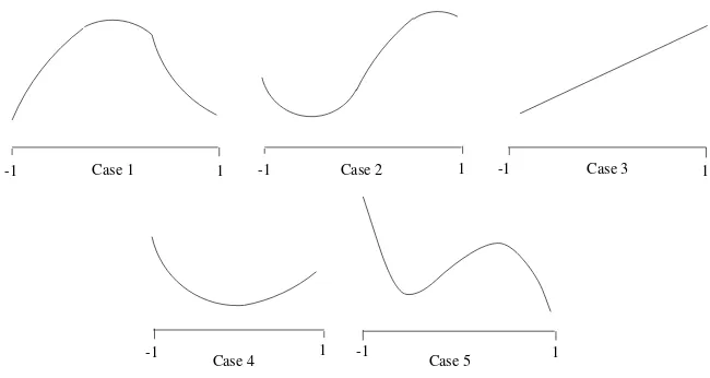
such thatfx(˜x) = 0butx˜is not optimal. More generally, any one of the five cases in Table 2.1 may occur. The diagrams in Figure 2.1 illustrate these cases. In each caseΩ = (−1,1).
2.4. REMARKS AND EXTENSIONS 13
Case 1 Case 2 Case 3
Case 5 Case 4
-1 1 -1 1
-1 1 1
-1 -1 1
Figure 2.2: Illustration of 4.1.
2.4.2 Existence.
If the set of permissible decisions Ωis a closed and bounded subset ofRn, and iff is continuous, then it follows by the Weierstrass Theorem that there exists an optimal decision. But ifΩisclosed we cannot assert that the derivative off vanishes at the optimum. Indeed, in the third figure above, ifΩ = [−1,1], then +1 is the optimal decision but the derivative is positive at that point.
2.4.3 Local optimum.
We say thatx∗ ∈ Ω is a locally optimal decision if there existsε > 0 such that f(x∗) ≥ f(x)
wheneverx ∈ Ωand |x∗ −x| ≤ ε. It is easy to see that the theorem holds(i.e., 2.11) for local
optima also.
2.4.4 Second-order conditions.
Supposefis twice-differentiable and letx∗ ∈Ωbe optimal or even locally optimal. Thenfx(x∗) =
0, and by Taylor’s theorem
f(x∗+δh) =f(x∗) +1
2δ2h′fxx(x∗)h+o(δ2), (2.20) where o(δδ22) →0asδ→0. Now forδ >0sufficiently smallf(x∗+δh)≤f(x∗), so that dividing
byδ2 >0yields
0≥ 12h′f
xx(x∗)h+ o(δ
2
) δ2
and letting δ approach zero we conclude that h′f
xx(x∗)h ≤ 0 for all h ∈ Rn. This means that
fxx(x∗)is a negative semi-definite matrix. Thus, if we have a twice differentiable objective function, we get an additional necessary condition.
2.4.5 Sufficiency for local optimal.
Suppose atx∗ ∈ Ω, f
2.4.6 A numerical procedure.
At any pointx˜∈Ωthe gradient▽xf(˜x)is a direction along whichf(x)increases,i.e.,f(˜x+ε▽x f(˜x))> f(˜x)for allε >0sufficiently small. This observation suggests the following scheme for finding a pointx∗ ∈Ωwhich satisfies 2.11. We can formalize the scheme as an algorithm.
Step 1. Pickx0 ∈Ω. Seti= 0. Go to Step 2. Step 2. Calculate▽xf(xi). If▽xf(xi) = 0, stop.
Otherwise letxi+1 =xi+di▽xf(xi)and go to Step 3.
Step 3. Seti=i+ 1and return to Step 2.
The step sizedi can be selected in many ways. For instance, one choice is to take di to be an optimal decision for the following problem:
Max{f(xi+d▽xf(xi))|d >0,(xi+d▽xf(xi))∈Ω}.
This requires a one-dimensional search. Another choice is to let di = di−1 iff(xi +di−1 ▽x
f(xi)) > f(xi); otherwise letd
i = 1/k di−1 where k is the smallest positive integer such that
f(xi+ 1/k d
i−1▽xf(xi))> f(xi). To start the process we letd−1 >0be arbitrary.
Exercise:Letf be continuous differentiable. Let{di}be produced by either of these choices and let
{xi}be the resulting sequence. Then 1. f(xi+1)> f(xi)ifxi+16=xi, i
2. ifx∗ ∈Ωis a limit point of the sequence{xi}, fx(x∗) = 0.
Chapter 3
OPTIMIZATION OVER SETS
DEFINED BY EQUALITY
CONSTRAINTS
We first study a simple example and examine the properties of an optimal decision. This will generalize to a canonical problem, and the properties of its optimal decisions are stated in the form of a theorem. Additional properties are summarized in Section 3 and a numerical scheme is applied to determine the optimal design of resistive networks.
3.1
Example
We want to find the rectangle of maximum area inscribed in an ellipse defined by
f1(x, y) = x
2
a2 +
y2
b2 =α. (3.1)
The problem can be formalized as follows (see Figure 3.1):
Maximize subject to
f0(x, y)
(x, y)∈Ω
= 4xy
={(x, y)|f1(x, y) =α}.
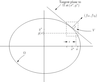
(3.2) The main difference between problem (3.2) and the decisions studied in the last chapter is that the set of permissible decisionsΩisnotan open set. Hence, if(x∗, y∗)is an optimal decision we cannotassert thatf0(x∗, y∗) ≥f0(x, y)for all(x, y)in an open set containing(x∗, y∗).Returning to problem (3.2), suppose(x∗, y∗)is an optimal decision. Clearly then eitherx∗6= 0ory∗6= 0.Let
us supposey∗ 6= 0.Then from figure 3.1 it is evident that there exist (i)ε >0,(ii) an open setV
containing(x∗, y∗),and (iii) a differentiable functiong: (x∗−ε, x∗+ε)→V such that
f1(x, y) =α and (x, y)∈V iff f y=g(x).1 (3.3) In particular this implies thaty∗ =g(x∗),and thatf1(x, g(x)) =αwhenever|x−x∗|< ε.Since
1Note thaty∗6= 0impliesf
1y(x∗, Y∗)6= 0,so that this assertion follows from the Implicit Function Theorem. The
assertion is false ify∗= 0.In the present case let0< ε≤a−x∗andg(x) = +b[α−(x/a)2
]1/2
.
) ( |
-y∗ g(x)
Tangent plane to
Ωat(x∗, y∗)
(f1x, f1y)
V
ǫ
x∗ x
Ω
Figure 3.1: Illustration of example.
(x∗, y∗) = (x∗, g(x∗))is optimum for (3.2), it follows thatx∗is an optimal solution for (3.4): Maximize
subject to
ˆ
f0(x) =f0(x, g(x))
|x−x∗|< ε. (3.4)
But the constraint set in (3.4) is an open set (inR1) and the objective functionfˆ0 is differentiable, so that by Theorem 2.3.1,fˆ0x(x∗) = 0, which we can also express as
f0x(x∗, y∗) +f0y(x∗, y∗)gx(x∗) = 0 (3.5) Using the fact thatf1(x, g(x))≡αfor|x−x∗|< ε, we see that
f1x(x∗, y∗) +f1y(x∗, y∗)gx(x∗) = 0,
and sincef1y(x∗, y∗)6= 0we can evaluategx(x∗),
gx(x∗) =−f1y−1f1x(x∗, y∗),
and substitute in (3.5) to obtain the condition (3.6):
f0x−f0yf1y−1f1x = 0 at (x∗, y∗). (3.6) Thus an optimal decision(x∗, y∗)must satisfy the two equationsf
1(x∗, y∗) =αand (3.6). Solving these yields
3.2. GENERAL CASE 17 Evidently there are two optimal decisions,(x∗, y∗) = −+(α/2)1/2(a, b), and the maximum area is
m(α) = 2αab. (3.7)
The condition (3.6) can be interpreted differently. Define
λ∗=f
0yf1y−1(x∗, y∗). (3.8)
Then (3.6) and (3.8) can be rewritten as (3.9):
(f0x, f0y) =λ∗(f1x, f1y) at (x∗, y∗) (3.9) In terms of the gradients off0, f1, (3.9) is equivalent to
▽f0(x∗, y∗) = [▽f1(x∗, y∗)]λ∗, (3.10) which means that at an optimal decision the gradient of the objective function f0 is normal to the plane tangent to the constraint setΩ.
Finally we note that
λ∗ = ∂m
∂α. (3.11)
wherem(α) =maximum area.
3.2
General Case
3.2.1 Theorem.
Letfi :Rn→R, i= 0,1, . . . , m (m < n), be continuously differentiable functions and letx∗ be an optimal decision of problem (3.12):
Maximize subject to
f0(x)
fi(x) =αi, i= 1, . . . , m.
(3.12) Suppose that atx∗the derivativesfix(x∗), i= 1, . . . , m,arelinearly independent. Then there exists a vectorλ∗= (λ∗1, . . . , λ∗m)′such that
f0x(x∗) =λ∗1f1x(x∗) +. . .+λ∗mfmx(x∗) (3.13) Furthermore, letm(α1, . . . , αm)be the maximum value of (3.12) as a function ofα = (α1, . . . , αm)′. Letx∗(α)be an optimal decision for (3.12). Ifx∗(α)is adifferentiable function ofαthenm(α)is a differentiable function ofα, and
(λ∗)′= ∂m∂α (3.14)
Proof.Sincefix(x∗), i= 1, . . . , m,are linearly independent, then by re-labeling the coordinates of
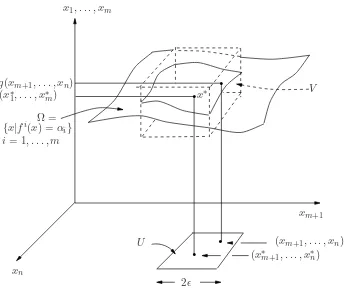
open set V in Rn containing x∗, and (iii) a differentiable function g : U → Rm, where U = [(xm+1, . . . , xn)]| |xm+ℓ−x∗m+ℓ|< ε, ℓ= 1, . . . , n−m], such that
fi(x1, . . . , xn) =αi,1≤i≤m, and (x1, . . . , xn)∈V iff
xj =gj(xm+1, . . . , xn),1≤j ≤m, and (xm+1, . . . , xn)∈U (3.15) (see Figure 3.2).
In particular this implies thatx∗
j =gj(x∗m+1, . . . , x∗n),1≤j≤m, and
fi(g(xm+1, . . . , xn), xm+1, . . . , xn) =αi , i= 1, . . . , m. (3.16) For convenience, let us definew = (x1, . . . , xm)′, u = (xm+1, . . . , xn)′ and f = (f1, . . . , fm)′. Then, since x∗ = (w∗, u∗) = (g(u∗), u∗) is optimal for (3.12), it follows that u∗ is an optimal decision for (3.17):
Maximize subject to
ˆ
f0(u) =f0(g(u), u)
u∈U. (3.17)
But U is an open subset of Rn−m and fˆ0 is a differentiable function on U (since f0 and g are differentiable), so that by Theorem 2.3.1 ,fˆ0u(u∗) = 0, which we can also express using the chain rule for derivatives as
ˆ
f0u(u∗) =f0w(x∗)gu(u∗) +f0u(x∗) = 0. (3.18) Differentiating (3.16) with respect tou= (xm+1, . . . , xn)′, we see that
fw(x∗)gu(u∗) +fu(x∗) = 0,
and since them×mmatrixfw(x∗)is nonsingular we can evaluategu(u∗),
gu(u∗) =−[fw(x∗)]−1fu(x∗),
and substitute in (3.18) to obtain the condition
−f0wfw−1fu+f0u = 0 at x∗ = (w∗, u∗). (3.19) Next, define the m-dimensional column vectorλ∗by
(λ∗)′ =f0wfw−1|x∗. (3.20) Then (3.19) and (3.20) can be written as (3.21):
(f0w(x∗), f0u(x∗)) = (λ∗)′(fw(x∗), fu(x∗)). (3.21) Sincex= (w, u), this is the same as
3.2. GENERAL CASE 19
.
.
.
.
x1, . . . , xm
x∗ V
xm+1
(xm+1, . . . , xn)
(x∗m+1, . . . , x∗n)
2ǫ U
xn
Ω =
{x|fi(x) =αi} i= 1, . . . , m
(x∗1, . . . , x∗m)
g(xm+1, . . . , xn)
Figure 3.2: Illustration of theorem.
which is equation (3.13).
To prove (3.14), we vary α in a neighborhood of a fixed value, say α. We define w∗(α) =
(x∗1(α), . . . , xm∗ (α))′ and u∗(α) = (x∗m+1(α), . . . , x∗(α))′. By hypothesis, fw is nonsingular at
x∗(α). Sincef(x) and x∗(α) are continuously differentiable by hypothesis, it follows thatfw is nonsingular atx∗(α)in a neighborhood ofα, sayN. We have the equation
f(w∗(α), u∗(α)) =α, (3.22)
−f0wfw−1fu+f0u = 0 at (w∗(α), u∗(α)), (3.23) forα∈N. Also,m(α) =f0(x∗(α)), so that
mα=f0ww∗α+f0uu∗α (3.24)
Differentiating (3.22) with respect toαgives
fww∗α+fuu∗α =I,
so that
and multiplying on the left byf0w gives
f0ww∗α+f0wfw−1fuu∗α=f0wfw−1.
Using (3.23), this equation can be rewritten as
f0wwα∗ +f0uuα∗ =f0wfw−1. (3.25) In (3.25), if we substitute from (3.20) and (3.24), we obtain (3.14) and the theorem is proved. ♦
3.2.2 Geometric interpretation.
The equality constraints of the problem in 3.12 define an−mdimensional surface
Ω ={x|fi(x) =αi, i= 1, . . . , m}.
The hypothesis of linear independence of{fix(x∗)|1 ≤i ≤m}guarantees that the tangent plane throughΩatx∗is described by
{h|fix(x∗)h= 0 , i= 1, . . . , m}, (3.26)
so that the set of (column vectors orthogonal to this tangent surface is
{λ1▽xf1(x∗) +. . .+λm▽xfm(x∗)|λi ∈R, i= 1, . . . , m}.
Condition (3.13) is therefore equivalent to saying that at an optimal decisionx∗, the gradient of the objective function▽xf0(x∗)is normal to the tangent surface (3.12).
3.2.3 Algebraic interpretation.
Let us again define w = (x1, . . . , xm)′ andu = (xm+1, . . . , xn)′. Suppose that fw(˜x)is nonsin-gular at some pointx˜ = ( ˜w,u˜)inΩwhich is not necessarily optimal. Then the Implicit Function Theorem enables us to solve, in a neighborhood ofx˜, themequationsf(w, u) =α.ucan then vary arbitrarilyin a neighborhood ofu˜. Asuvaries,wmust change according tow=g(u)(in order to maintainf(w, u) = α), and the objective function changes according tofˆ0(u) =f0(g(u), u). The derivative offˆ0atu˜is
ˆ
f0u(˜u) =f0wgu+f0u˜x=−λ˜′fu(˜x) +f0u(˜x),
where
˜
λ′ =f0wfw˜−x1, (3.27)
Therefore,the direction of steepest increase offˆ0atu˜is
3.3. REMARKS AND EXTENSIONS 21
3.3
Remarks and Extensions
3.3.1 The condition of linear independence.
The necessary condition (3.13) need not hold if the derivativesfix(x∗),1≤i≤m, are not linearly independent. This can be checked in the following example
Minimize
subject to sin(x21+x22)
π
2(x21+x22) = 1.
(3.29)
3.3.2 An alternative condition.
Keeping the notation of Theorem 3.2.1, define the Lagrangian functionL : Rn+m → R byL : (x, λ) 7→ f0(x)−Pmi=1λifi(x). The following is a reformulation of 3.12, and its proof is left as an exercise.
Let x∗ be optimal for (3.12), and suppose thatfix(x∗),1 ≤ i ≤ m, are linearly independent. Then there existsλ∗ ∈Rm such that(x∗, λ∗)is astationary point ofL, i.e.,Lx(x∗, λ∗) = 0and
Lλ(x∗, λ∗) = 0.
3.3.3 Second-order conditions.
Since we can convert the problem (3.12) into a problem of maximizing fˆ0 over an open set, all the comments of Section 2.4 will apply to the functionfˆ0. However, it is useful to translate these remarks in terms of the original function f0 and f. This is possible because the function g is uniquely specified by (3.16) in a neighborhood ofx∗. Furthermore, iff is twice differentiable, so isg (see Fleming [1965]). It follows that if the functions fi,0 ≤ i ≤ m, are twice continuously differentiable, then so isfˆ0, and a necessary condition forx∗to be optimal for (3.12) and (3.13) and the condition that the(n−m)×(n−m)matrixfˆ0uu(u∗)is negative semi-definite. Furthermore, if this matrix is negative definite then x∗ is a local optimum. the following exercise expresses
ffˆ0uu(u∗)in terms of derivatives of the functionsfi.
Exercise:Show that
ˆ
f0uu(u∗) = [g′u...I]
Lww
Luw
Lwu
Luu
gu
. . . I
(w∗, u∗)
where
gu(u∗) =−[fw(x∗)]−1fu(x∗), L(x) =f0(x)− m
X
i=1
3.3.4 A numerical procedure.
We assume that the derivatives fix(x),1 ≤ i ≤ m, are linearly independent for allx. Then the following algorithm is a straightforward adaptation of the procedure in Section 2.4.6.
Step 1. Findx0arbitrary so thatfi(x0) =αi,1≤i≤m. Setk= 0and go to Step 2. Step 2. Find a partitionx= (w, u)2of the variables such thatf
w(xk)is nonsingular. Calculateλk by(λk)′ =f
0wfw(xk)−1 , and▽fˆ0k(uk) =−fu′(xk)λk+f0u′ (xk). If▽fˆ0k(uk) = 0,stop. Otherwise go to Step 3.
Step 3. Setu˜k=uk+dk▽fˆ0k(uk). Findw˜ksuch thatfi( ˜wk,u˜k) = 0,1≤i≤m. Set
xk+1 = ( ˜wk,u˜k), setk=k+ 1, and return to Step 2.
Remarks.As before, the step sizesdk>0can be selected various ways. The practical applicability of the algorithm depends upon two crucial factors: the ease with which we can find a partition
x= (w, u)so thatfw(xk)is nonsingular, thus enabling us to calculateλk; and the ease with which we can findw˜kso thatf( ˜wk,u˜k) =α. In the next section we apply this algorithm to a practical problem where these two steps can be carried out without too much difficulty.
3.3.5 Design of resistive networks.
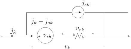
Consider a network N withn+ 1 nodes andb branches. We choose one of the nodes as datum and denote bye = (e1, . . . , en)′ the vector of node-to-datum voltages. Orient the network graph and letv = (v1, . . . , vb)′ andj = (j1, . . . , jb)′ respectively, denote the vectors of branch voltages and branch currents. LetAbe then×breduced incidence matrix of the network graph. Then the Kirchhoff current and voltage laws respectively yield the equations
Aj = 0 and A′e=v (3.30)
Next we suppose that each branchkcontains a (possibly nonlinear)resistive element with the form shown in Figure 3.3, so that
jk−jsk=gk(vrk) =gk(vk−vsk),1≤k≤b, (3.31) wherevrkis the voltage across the resistor. Herejsk,vskare the source current and voltage in the kthbranch, andgk is the characteristic of the resistor. Using the obvious vector notationjs ∈Rb,
vs ∈ Rb for the sources,vr ∈ Rb for the resistor voltages, andg = (g1, . . . , gb)′, we can rewrite (3.30) as (3.31):
j−js=g(v−vs) =g(vr). (3.32)
Although (3.30) implies that the current (jk−jsk) through thekthresistor depends only on the voltage vrk = (vk−vsk)across itself, no essential simplification is achieved. Hence, in (3.31) we shall assume that gk is a function of vr. This allows us to include coupled resistors and voltage-controlled current sources. Furthermore, let us suppose that there are ℓ design parameters p = (p1, . . . , pℓ)′ which are under our control, so that (3.31) is replaced by (3.32):
j−jx=g(vr, p) =g(v−vs, p). (3.33)
3.3. REMARKS AND EXTENSIONS 23
o
-+ - +
-+
o jsk
vrk
vsk
jk−jsk
jk
[image:31.612.197.416.83.166.2]vk
Figure 3.3: Thekth branch.
If we combine (3.29) and (3.32) we obtain (3.33):
Ag(A′e−vs, p) =is, (3.34)
where we have definedis=Ajs. The network design problem can then be stated as findingp, vs, is so as to minimize some specified functionf0(e, p, vs, is). Formally, we have the optimization prob-lem (3.34):
Minimize subject to
f0(e, p, vs, is)
Ag(A′e−vs, p)−is = 0.
(3.35) We shall apply the algorithm 3.3.4 to this problem. To do this we make the following assumption.
Assumption: (a)f0is differentiable. (b)gis differentiable and then×nmatrixA(∂g/∂v)(v, p)A′ is nonsingular for allv ∈Rb, p ∈ Rℓ. (c) The networkN described by (3.33) is determinatei.e., for every value of(p, vs, is)there is a uniquee=E(p, vs, is)satisfying (3.33).
In terms of the notation of 3.3.4, if we let x = (e, p, vs, is), then assumption (b) allows us to identifyw=e, andu= (p, vs, is). Also letf(x) =f(e, p, vs, is) =Ag(A′e−vs, p)−is. Now the crucial part in the algorithm is to obtainλkat some pointxk. To this end letx˜= (˜e,p,˜ v˜
s,˜is)be a fixed point. Then the correspondingλ= ˜λis given by (see (3.27))
˜
λ′ =f
0w(˜x)fw−1(˜x) =f0e(˜x)fe−1(˜x). (3.36) From the definition off we have
fe(˜x) =AG(˜vr,p˜)A′,
wherev˜r = A′e˜−v˜s, and G(˜vr,p˜) = (∂g/∂vr)(˜vr,p˜). Therefore, ˜λis the solution (unique by assumption (b)) of the following linear equation:
AG′(˜v
r,p˜)A′λ˜=f0e′ (˜x). (3.37) Now (3.36) has the following extremely interesting physical interpretation. If we compare (3.33) with (3.36) we see immediately that ˜λis the node-to-datum response voltages of alinearnetwork
N(˜vr,p˜) driven by the current sources f0e′ (˜x). Furthermore, this network has the samegraph as the original network (since they have the same incidence matrix); moreover, its branch admittance matrix,G′(˜v
Once we have obtained λ˜ we can obtain ▽ufˆ0(˜u)using (3.28). Elementary calculations yield (3.37):
▽ufˆ0(˜u) =
ˆ
f0p′ (˜u) ˆ
f′
0vs(˜u)
ˆ
f0is′ (˜u)
=
[∂g∂p(˜vr,p˜)]′A′
G′(˜vr,p˜)A′ −I λ˜ + f′
0p(˜x)
f′
0vs(˜x)
f0is′ (˜x)
(3.38)
We can now state the algorithm. Step 1. Selectu0 = (p0, v0
s, i0s)arbitrary. Solve (3.33) to obtaine0=E(p0, vs0, i0s). Letk= 0and go to Step 2.
Step 2. Calculatevk
r =A′ek−vsk. calculatef0e′ (xk). Calculate the node-to-datum responseλkof the adjoint networkN(vrk, pk)driven by the current sourcef0e′ (xk). Calculate▽ufˆ0(uk)from (3.37). If this gradient is zero, stop. Otherwise go to Step 3.
Step 3. Letuk+1= (pk+1, vk+1
s , ik+1s ) =uk−dk▽ufˆ0(uk), wheredk>0is a predetermined step size. 3 Solve (3.33) to obtainek+1 = (Epk+1, vsk+1, ik+1s ). Setk=k+ 1and return to Step 2. Remark 1.Each iteration fromuktouk+1requires one linear network analysis step (the
computation ofλkin Step 2), and one nonlinear network analysis step (the computation ofek+1in step 3). This latter step may be very complex.
Remark 2.In practice we can control only some of the components ofvsandis, the rest being fixed. The only change this requires in the algorithm is that in Step 3 we set
pk+1 =pk−dkfˆ0p′ (uk)just as before, where asvsjk+1 =vksj−dk(∂fˆ0/∂vsj)(uk)and
ik+1
sm =iksm−dk(∂fˆ0/∂ism)(uk)withjandmranging only over the controllable components and the rest of the components equal to their specified values.
Remark 3.The interpretation ofλas the response of the adjoint network has been exploited for particular functionf0in a series of papers (director and Rohrer [1969a], [1969b], [1969c]). Their derivation of the adjoint network does not appear as transparent as the one given here. Although we have used the incidence matrixAto obtain our network equation (3.33), one can use a more general cutset matrix. Similarly, more general representations of the resistive elements may be employed. In every case the “adjoint” network arises from a network interpretation of (3.27),
[fw(˜x)]′λ˜ =f0w(˜x),
with the transpose of the matrix giving rise to the adjective “adjoint.”
Exercise:[DC biasing of transistor circuits (see Dowell and Rohrer [1971]).] LetN be a transistor circuit, and let (3.33) model the dc behavior of this circuit. Suppose thatisis fixed,vsj forj∈J are variable, andvsj forj /∈Jare fixed. For each choice ofvsj,j∈J, we obtain the vectoreand hence the branch voltage vectorv=A′e. Some of the componentsvt, t∈T, will correspond to bias voltages for the transistors in the network, and we wish to choosevsj, j ∈J, so thatvtis as close as possible to a desired bias voltagevdt, t∈T. If we choose nonnegative numbersαt, with relative magnitudes reflecting the importance of the different transistors then we can formulate the criterion
3Note the minus sign in the expressionuk−d
k▽ufˆ0(uk). Remember we are minimizingf0, which is equivalent to
3.3. REMARKS AND EXTENSIONS 25
f0(e) =
X
t∈T
αt|vt−vdt|2.
(i) Specialize the algorithm above for this particular case.
Chapter 4
OPTIMIZATION OVER SETS
DEFINED BY INEQUALITY
CONSTRAINTS: LINEAR
PROGRAMMING
In the first section we study in detail Example 2 of Chapter I, and then we define the general linear programming problem. In the second section we present the duality theory for linear program-ming and use it to obtain some sensitivity results. In Section 3 we present the Simplex algorithm which is the main procedure used to solve linear programming problems. In section 4 we apply the results of Sections 2 and 3 to study the linear programming theory of competitive economy. Additional miscellaneous comments are collected in the last section. For a detailed and readily ac-cessible treatment of the material presented in this chapter see the companion volume in this Series (Sakarovitch [1971]).
4.1
The Linear Programming Problem
4.1.1 Example.
Recall Example 2 of Chapter I. Letgandurespectively be the number of graduate and undergradu-ate students admitted. Then the number of seminars demanded per year is 2g+u20 , and the number of lecture courses demanded per year is 5g+7u40 . On the supply side of our accounting, the faculty can offer2(750) + 3(250) = 2250seminars and6(750) + 3(250) = 5250lecture courses. Because of his contractual agreements, the President must satisfy
2g+u
20 ≤2250or2g+u≤45,000 and
5g+7u
Since negativegoruis meaningless, there are also the constraintsg≥0, u≥0. Formally then the President faces the following decision problem:
Maximize αg+βu
subject to 2g+u≤45,000 5g+ 7u≤210,000
g≥0, u≥0.
(4.1)
It is convenient to use a more general notation. So letx= (g, u)′, c= (α, β)′, b= (45000,210000,0,0)′
and letAbe the 4×2 matrix
A=
2 5
−1 0
1 7 0
−1
.
Then (4.1) can be rewritten as (4.2)1
Maximizec′x
subject toAx≤b . (4.2)
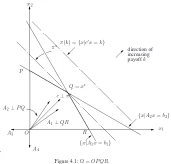
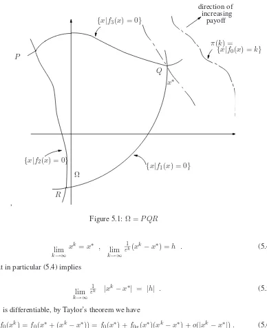
LetAi,1≤i≤4, denote therowsofA. Then the setΩof all vectorsxwhich satisfy the constraints in (4.2) is given byΩ ={x|Aix≤bi, 1≤i≤4}and is the polygonOP QRin Figure 4.1.
For each choicex, the President receives the payoffc′x. Therefore, the surface of constant payoff
k say, is the hyperplane π(k) = {x|c′x = k}. These hyperplanes for different values of k are parallel to one another since they have the same normalc. Furthermore, askincreasesπ(k)moves in the directionc. (Obviously we are assuming in this discussion thatc6= 0.) Evidently an optimal decision is any pointx∗ ∈Ωwhich lies on a hyperplaneπ(k)which is farthest along the direction
c. We can rephrase this by saying thatx∗ ∈ Ωis an optimal decision if and only if the planeπ∗
throughx∗ does not intersect the interior of Ω, and futhermore atx∗ the direction cpoints away fromΩ. From this condition we can immediately draw two very important conclusions: (i) at least one of the vertices of Ωis an optimal decision, and (ii) x∗ yields a higher payoff than all points
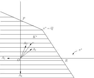
in the coneK∗consisting of all rays starting at x∗ and passing through Ω, sinceK∗ lies “below”
π∗. The first conclusion is the foundation of the powerful Simplex algorithm which we present in Section 3. Here we pursue consequences of the second conclusion. For the situation depicted in Figure 4.1 we can see thatx∗ =Qis an optimal decision and the coneK∗ is shown in Figure 4.2. Nowx∗satisfiesAxx∗ =b1, A2x∗ =b2, andA3x∗< b3, A4x∗ < b4, so thatK∗is given by
K∗={x∗+h|A1h≤0, A2h≤0}.
Sincec′x∗ ≥c′yfor ally∈K∗ we conclude that
c′h≤0 for all h such that A1h≤0, A2h≤0. (4.3) We pause to formulate the generalization of (4.3) as an exercise.
1Recall the notation introduced in 1.1.2, so thatx≤ymeansx
4.1. THE LINEAR PROGRAMMING PROBLEM 29
,
-x2
π(k) ={x|c′x=k} π∗
Q=x∗
direction of increasing payoffk
{x|A2x=b2}
x1
{x|A1x=b1}
R
A4
O A3
A1 ⊥QR
c⊥π∗
A2 ⊥P Q
[image:37.612.142.484.81.409.2]P
Figure 4.1:Ω =OP QR.
Exercise 1: LetAi, 1≤i≤k, ben-dimensionalrowvectors. Letc∈Rn, and letbi, 1≤i≤k, be real numbers. Consider the problem
Maximizec′x
subject toAix≤bi, 1≤i≤k .
For anyxsatisfying the constraints, letI(x)⊂ {1, . . . , n}be such thatAi(x) =bi, i∈I(x), Aix <
bi, i /∈I(x). Supposex∗satisfies the constraints. Show thatx∗is optimal if an only if
c′h≤0for all hsuch thatA
ih≤0, i∈I(x∗).
Returning to our problem, it is clear that (4.3) is satisfied as long as clies betweenA1 and A2. Mathematically this means that (4.3) is satisfied if and only if there existλ∗1≥0, λ∗2≥0such that
2
c′=λ∗
1, A1+λ∗2A2. (4.4)
Ascvaries, the optimal decision will change. We can see from our analysis that the situation is as follows (see Figure 4.1):
2Although this statement is intuitively obvious, its generalization tondimensions is a deep theorem known as Farkas’
P
x∗ =Q
K∗
π∗
R
A4
O A3
A2 c
[image:38.612.146.467.82.349.2]A1
Figure 4.2:K∗is the cone generated byΩatx∗.
1. x∗ =Qis optimal iffclies betweenA1andA2iffc′=λ1∗A1+λ∗2A2for someλ∗1 ≥0, λ∗2≥
0,
2. x∗ ∈QP is optimal iffclies alongA2iffc′ =λ∗2A2 for someλ∗2 ≥0, 3. x∗ =P is optimal iffclies betweenA
3andA2iffc′ =λ∗2A2+λ∗3A3for someλ∗2≥0, λ∗3≥
0,etc.
These statements can be made in a more elegant way as follows:
x∗∈Ωis optimal iff there existsλ∗i ≥0, 1≤i≤4, such that
(a) c′ =
4
X
i=1
λ∗iai, (b) ifAi x∗ < bi thenλ∗i = 0. (4.5) For purposes of application it is useful to separate those constraints which are of the formxi ≥0, from the rest, and to reformulate (4.5) accordingly We leave this as an exercise.
Exercise 2:Show that (4.5) is equivalent to (4.6), below. (HereAi = (ai1, ai2).)x∗ ∈Ωis optimal iff there existλ∗
1 ≥0, λ∗2 ≥0 such that
(a) ci≤λ∗1a1i+λ∗2a2i, i= 1, 2,
(b) ifaj1x∗1+aj2x∗2< bj thenx∗j = 0, j= 1,2.
(c) ifci< λ∗1i+λ2∗a2i thenx∗i = 0, i= 1,2.
4.1. THE LINEAR PROGRAMMING PROBLEM 31
4.1.2 Problem formulation.
A linear programming problem (or LP in brief) is any decision problem of the form 4.7.
Maximizec1x1+c2x2+. . .+cnxn subject to
ailx1+ai2x2+. . .+ainxn≤ bi , l≤i≤k ,
ailx1+. . . .+ainxn ≥ bi , k+ 1≤i≤ℓ ,
ailx1+. . . .+ainxn = bi , ℓ+ 1≤i≤m ,
and
xj ≥0 , 1≤j≤p ,
xj ≥0 , p+ 1≤j≤q;
xj arbitary, q+ 1≤j≤n ,
(4.7)
where thecj, aij, biare fixed real numbers. There are two important special cases: Case I:(4.7) is of the form (4.8):
Maximize n
X
j=1
cjxj
subject to n
X
j=1
aijxj ≤bi,
xj ≥0 ,
1≤i≤m ,
1≤j≤n
(4.8)
Case II:(4.7) is of the form (4.9):
Maximize n
X
j=1
cjxj
subject to n
X
j=1
aijxj =bi,
xj ≥0 ,
1≤i≤m ,
1≤j≤n .
(4.9)
Although (4.7) appears to be more general than (4.8) and (4.9), such is not the case.
Proposition: Every LP of the form (4.7) can be transformed into an equivalent LP of the form (4.8). Proof.
Step 1:Replace each inequality constraintP
aijxj ≥bibyP(−aij)xj ≤(−bi). Step 2:Replace each equality constraintP
aijxj =biby two inequality constraints:
P
aijxj ≤bi, P(−aij)xj ≤(−bi).
Step 3:Replace each variablexjwhich is constrainedxj ≤0by a variableyj =−xjconstrained
Step 4:Replace each variablexjwhich is not constrained in sign by a pair of variables
yj−zj =xj constrainedyj ≥0, zj ≥0and then replaceaijxjbyaijyj+ (−aij)zj for everyiand
cjxj bycjyj+ (−cj)zj. Evidently the resulting LP has the form (4.8) and is equivalent to the
original one. ♦
Proposition: Every LP of the form (4.7) can be transformed into an equivalent LP of the from (4.9) Proof.
Step 1:Replace each inequality constraintP
aijxj ≤biby the equality constraint
P
aijxj+yi=bi whereyiis an additional variable constrainedyi≥0. Step 2:Replace each inequality constraintP
aijxj ≥biby the equality constraint
P
aijxj−yi=bi whereyiis an additional variable constrained byyi ≥0. (The new variables added in these steps are calledslackvariables.)
Step 3, Step 4: Repeat these steps from the previous proposition. Evidently the new LP has the
form (4.9) and is equivalent to the original one. ♦
4.2
Qualitative Theory of Linear Programming
4.2.1 Main results.
We begin by quoting a fundamental result. For a proof the reader is referred to (Mangasarian [1969]).
Farkas’ Lemma.LetAi, 1≤i≤k, ben-dimensionalrowvectors. Letc∈Rnbe a column vector. The following statements are equivalent:
(i) for allx∈Rn, Aix≤0for1≤i≤kimpliesc′x≤0, (ii) there existsλ1≥0, . . . , λk ≥0such thatc′ =
k
X
i=1
λiAi. An algebraic version of this result is sometimes more convenient.
Farkas’ Lemma (algebraic version). LetAbe ak×nmatrix. Letc∈Rn. The following statements are equivalent.
(i) for allx∈Rn, Ax≤0impliesc′x≤0,
(ii) there existsλ≥0, λ∈Rk,such thatA′λ=c.
Using this result it is possible to derive the main results following the intuitive reasoning of (4.1). We leave this development as two exercises and follow a more elegant but less intuitive approach.
Exercise 1: With the same hypothesis and notation of Exercise 1 in 4.1, use the first version of Farkas′ lemma to show that there existλ∗i ≥0fori∈I(x∗)such that X
i∈I(x∗)
λ∗iAi =c′ .
Exercise 2: Letx∗satisfy the constraints for problem (4.17). Use the previous exercise to show
thatx∗is optimal iff there existλ∗
1≥0, . . . , λ∗m≥0such that (a) cj ≤
m
X
i=1
λ∗iaij , 1≤j≤n
(b) if n
X
j=1
aijx∗j < bithenλ∗i = 0, 1≤i≤m(c) if m
X
i=1
λ∗iaij > cj thenx∗j = 0, 1≤j≤m.
In the remaining discussion, c ∈ Rn, b ∈n are fixed vectors, andA = {a
4.2. QUALITATIVE THEORY OF LINEAR PROGRAMMING 33 below. (4.10) is called theprimalproblem and (4.11) is called thedualproblem.
Maximize subject to
c1x1+. . .+cnxn
ai1x1+. . .+ainxn≤bi,
xj ≥0,
1≤i≤m
1≤j≤n .
(4.10)
Maximize subject to
λ1b1+. . .+λmbm
λ1a1j +. . .+λmamj ≥cj ,
λi ≥0,
1≤j≤n
1≤i≤m .
(4.11)
Definition: LetΩp ={x ∈Rn|Ax≤b, x≥0}be the set of all points satisfying the constraints of the primal problem. Similarly letΩd={λ∈Rm|λ′A≥c′, λ≥0}. A pointx∈Ωp(λ∈Ωd)is said to be afeasible solutionorfeasible decisionfor the primal (dual).
The next result is trivial.
Lemma 1:(Weak duality) Letx∈Ωp, λ∈Ωd. Then
c′x≤λ′Ax≤λ′b. (4.12)
Proof: x≥0andλ′A−c′ ≥0implies(λ′A−c′)x ≥0giving the first inequality. b−Ax≥0and
λ′≥0impliesλ′(b−Ax)≥0giving the second inequality. ♦ Corollary 1:Ifx∗∈Ωandλ∗ ∈Ω
dsuch thatc′x∗= (λ∗)′b, thenx∗is optimal for (4.10) andλ∗is optimal for (4.11).
Theorem 1: (Strong duality) SupposeΩp 6=φandΩd6=φ. Then there existsx∗ which is optimum for (4.10) andλ∗which is optimum for (4.11). Furthermore,c′x∗ = (λ∗)′b.
Proof: Because of the Corollary 1 it is enough to prove the last statement, i.e.,we must show that there exist x ≥ 0, λ ≥ 0, such thatAx ≤ b, A′λ ≥ cand b′λ−c′x ≤ 0. By introducing slack
variablesy ∈Rm, µ ∈Rm, r ∈R, this is equivalent to the existence ofx ≥0, y ≥0, λ≥0, µ≤
0, r≤0such that
A Im
A′ −I
n −c′ b′ 1
x y λ µ r = b c 0
By the algebraic version of Farkas’ Lemma, this is possible only if
A′ξ−cθ≤0 , ξ ≤0, Aw=bθ≤0 , −w≤0, θ≤0
(4.13)
implies
Case (i):Suppose(w, ξ, θ)satisfies (4.13) andθ <0. Then(ξ/θ)∈Ωd,(w/−θ)∈Ωp, so that by Lemma 1c′w/(−θ)≤b′ξ/θ, which is equivalent to (4.14) sinceθ <0.
Case (ii):Suppose(w, ξ, θ)satisfies (4.13) andθ= 0, so that−A′ξ≥0,−ξ ≥0,Aw≤0,w≥0. By hypothesis, there existx∈Ωp,λ∈Ωd. Hence,−b′ξ=b′(−ξ)≥(Ax)′(−ξ) =x′(−A′ξ)≥0, andc′w≤(A′λ)′w=λ′(Aw)≤0.So thatb′ξ+c′w≤0. ♦
The existence part of the above result can be strengthened.
Theorem 2:(i) SupposeΩp 6=φ. Then there exists an optimum decision for the primal LP iff
Ωd6=φ.
(ii) SupposeΩd6=φ. Then there exists an optimum decision for the dual LP iffΩp 6=φ. ProofBecause of the symmetry of the primal and dual it is enough to prove only (i). The sufficiency part of (i) follows from Theorem 1, so that only the necessity remains. Suppose, in contradiction, thatΩd=φ. We will show that sup{c′x|x∈Ωp}= +∞. Now,Ωd=φmeans there does not existλ≥0such thatA′λ≥c. Equivalently, there does not existλ≥0, µ≤0such
that
A′ |
| −In
λ
− − −
µ
=
c
By Farkas’ Lemma there existsw∈Rnsuch thatAw≤0,−w≤0, andc′w >0. By hypothesis,
Ωp 6= φ, so there exists x ≥ 0 such that Ax ≤ b. but then for anyθ > 0, A(x +θw) ≤ b,
(x +θw) ≥ 0, so that (x +θw) ∈ Ωp. Also, c′(x+θw) = c′x +θc′w. Evidently then, sup {c′x|x∈Ωp}= +∞so that there is no optimal decision for the primal. ♦
Remark:In Theorem 2(i), the hypothesis thatΩp6=φis essential. Consider the following exercise.
Exercise 3: Exhibit a pair of primal and dual problems such thatneitherhas a feasible solution. Theorem 3:(Optimality condition)x∗∈Ωp is optimal if and only if there existsλ∗ ∈Ωdsuch that
m
X
j=1
aijx∗j < biimpliesλ∗i = 0, and
m
X
i=1
λ∗iaij < cj impliesx∗j = 0.
(4.15)
((4.15) is known as the condition ofcomplementary slackness.)
Proof:First of all we note that forx∗ ∈Ωp,λ∗ ∈Ωd, (4.15) is equivalent to (4.16):
(λ∗)′(Ax∗−b) = 0, and(A′λ∗−c)′x∗ = 0. (4.16) Necessity. Supposex∗ ∈Ω
pis optimal. Then from Theorem 2,Ωd6=φ, so that by Theorem 1 there existsλ∗ ∈Ωdsuch thatc′x∗ = (λ∗)�