Jurnal Ekonomi dan Studi Pembangunan Volume 16, Nomor 1, April 2015, hlm.1-13
FACTORS INFLUENCING ECONOMIC GROWTH IN INDONESIA:
ERROR CORRECTION MODEL (ECM)
Yahya Muqorrobin
Institute of Public Policy and Economic Studies Jalan Kenari 13 Sidoarum III Yogyakarta, Indonesia
Correspondence E-mail: yahya.mq27@gmail.com
Received: Juli 2014; Accepted: February 2015
Abstract: The main objective of this study is to identify and analyze the effect of foreign direct investments (FDI), foreign debts, bank credit and labor force on the economic growth in Indonesia. Annual data during the period of 1985-2013 are used in this study and collected from Bank Indonesia, BKPM, and BPS. The study uses Error Correction Model (ECM). The result shows that foreign direct investment, bank credit and labor force positively and significantly influence the economic growth in Indonesia in short term and long term analyses. In the other hand, foreign debt negatively and significantly influences the economic growth in Indonesia in short term and long term.
Keywords: economic growth; foreign direct investment; foreign debt; bank credit; labor force
JEL Classification: F43, P45
Abstrak: Tujuan studi adalah mengidentifikasi dan menganalisis pengaruh penanaman modal asing (PMA), hutang luar negeri, kredit bank, dan angkatan kerja terhadap pertumbuhan ekonomi di Indonesia. Studi ini menggunakan data tahunan tahun 1985-2013 yang diperoleh dari Bank Indonesia, BKPM, dan BPS. Model yang digunakan dalam studi ini adalah Error Correction Model (ECM). Hasil studi menunjukkan bahwa penanaman modal asing, kredit bank, dan angkatan kerja berpengaruh positif dan signifikan terhadap pertumbuhan ekonomi di Indonesia dalam jangka pendek dan jangka panjang. Sebaliknya, hutang luar negeri berpengaruh negatif dan signifikan terhadap pertumbuhan ekonomi di Indonesia dalam jangka pendek dan jangka panjang.
Kata kunci: pertumbuhan ekonomi; penanaman modal asing; hutang luar negeri; kredit bank; angkatan kerja
Klasifikasi JEL: F43, P45
INTRODUCTION
Economic growth is one indicator that is very important in the analysis of economic develop-ment that occurs in a country. Economic growth shows the extent to which economic activity will generate additional income to the commu-nities in a given period. It is because economic activity is basically a process to produce output, measured with the GDP indicator.
Indonesia as a developing country tries to build the nation without expecting help from other countries. However it is difficult to
sur-vive in the middle of the swift currents of glob-alization that continue to grow rapidly. Under these conditions, Indonesia finally has to follow the flow by collaborating with other countries in the implementation of national development, especially the joint national economy.
eco-nomic growth rates fluctuated. However, at a certain point, the Indonesian economy finally collapses under the brunt of the economic crisis globally around the world. It is characterized by high rates of inflation, the value of the rupiah which continued to weaken, the high rate of unemployment, and coupled with the increas-ingly growing number of Indonesian foreign debt due to weaker exchange rate.
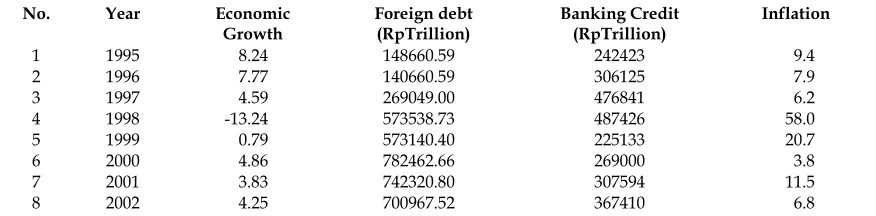
Since the crisis hit in the middle of 1997 it has become a big shock for the growth of the national economy. The monetary crisis affected the rate of economic growth in 1998 which experienced a minus of 13.1 percent and the increase of foreign debt from 269 trillion rupiah in 1997 to 573 trillion rupiah. Further indirect impacts of this crisis also hit the banking world one year later, when total bank credit in the form of consumption and capital declined from Rp487 trillion in 1998 to Rp225 trillion.
Indonesia's economic growth in 1999 starts growing positively despite only at the rate of 0.79 percent after a huge decline in 1998. Early signs of economic recovery has begun It seems, that monetary stability was under control, which was reflected in a low inflation rate and a stronger exchange rate, and political and social circumstances that have been more favorable.
A level of economic growth is determined, among others by the power of investment sector, foreign aid sector, and labor productiv-ity. Economic growth requires an increase in investment funds that in turn require funding from both domestic and abroad. From these two sources of financing, domestic sources should be the principal source of financing, especially viewed from the context in which the long-term economic growth of a country should
base their investment financing from domestic sources (Syaharani, 2011).
Because of the limited domestic resources owned while fund requirement for economic development is very large, and to overcome the lack of funds needed in the process of national development since Pelita I recent years, revenue funding is made from abroad, both in the form of foreign debt and foreign direct investment (FDI) (Kamaluddin, 2007).
The role of foreign aid and foreign capital to the progress, growth and economic devel-opment of developing countries has long been a heated debate among groups of the world economy. A group of economists in the 1950s and 1960s argued and believed that foreign aid has a positive impact on the economic devel-opment of a country without causing disruption in the aftermath of the debtor countries (Kam-aluddin, 2007).
For developing countries such as Indone-sia, the rapid flow of capital is a good oppor-tunity to obtain economic development financ-ing. However, if the funds are given through debt, then gradually foreign debts seem to be a boomerang for Indonesia because it leaves a lot of issues, especially foreign debts that have high interest rates. For a government, foreign debt payment is the largest consumption in the state budget in the last decade. While our country still has to pay for a wide range of other eco-nomic sectors that are also important and urgent (Anwar, 2011).
As an alternative to foreign debt, to get the funds from abroad can be done through Foreign Direct Investment (FDI). As well as with foreign debt, Foreign Direct Investment (FDI) is one of the sources of financing for
Table 1. Economic growth, foreign debt, banking credit and inflation in Indonesia 1995-2002
No. Year Economic
Growth
Foreign debt (RpTrillion)
Banking Credit (RpTrillion)
Inflation
1 1995 8.24 148660.59 242423 9.4
2 1996 7.77 140660.59 306125 7.9
3 1997 4.59 269049.00 476841 6.2
4 1998 -13.24 573538.73 487426 58.0
5 1999 0.79 573140.40 225133 20.7
6 2000 4.86 782462.66 269000 3.8
7 2001 3.83 742320.80 307594 11.5
8 2002 4.25 700967.52 367410 6.8
development and national economic growth. FDI is directed to replace the role of foreign debt to finance the growth and development of the national economy. The role of foreign capi-tal becomes even more crucial given the fact that the amount of Indonesia's foreign debt has increased significantly.
Foreign Direct Investment (FDI) destina-tion country is believed to be beneficial, espe-cially in terms of development and economic growth. Much empirical evidence such as the experiences in South Korea, Malaysia, Thailand, China, and many other countries shows that the presence of FDI gave a lot of positive things to the economy of the host country. In the case of Indonesia, the most obvious evidence is the past under the new order. Indonesian economy may not be able to rise again from the destruction created by the Old Order and could experience an average economic growth of 7 percent per year during the period of the 1980s when no FDI. Of course many other factors that also serve as a source of growth drivers such as aid or foreign debt and the seriousness of the New Order government to build a national economy when it is reflected by the presence of Repelita
and political and social stability. Literature the-ory also gives a strong argument that there is a positive correlation between FDI and economic growth in the recipient country (Tambunan, 2007).
The thought that supports that foreign capital has a positive effect on domestic savings and financing imports got a lot of challenges from the camp followers of dependency theory (dependencia). They concluded that only a small proportion of foreign capital has a posi-tive effect on domestic savings and economic growth. The main hypothesis is the dependency theory of FDI and foreign debt in the short-term that increase economic growth; more countries depend on FDI and foreign debt, so the differ-ence in earnings (income) becomes greater and in turn equity is not achieved (Anwar, 2011).
Foreign direct investment (FDI) is an alter-native to meet the development needs of capi-tal. In Indonesia, FDI regulated in the Act of Foreign Investment (UUPMA) which is a legal base of FDI to come to Indonesia. The Indone-sian government attempted to encourage the business climate so as to attract the interest of
private sector enterprises, especially for for-eigners, so the Act No. 1/1967 on Foreign Direct Investment (FDI) was issued. The Act was refined in 1970 to be Act No. 11/1970.
In addition to investment, labor is a factor that affects the output of a region. A large labor force will be formed from a large population. However, population growth could cause significant negative effects on economic growth. According to Todaro (2000) rapid population growth gave rise to the problem of under development and make the prospect of the development becomes increasingly distant. Further, it is said that the population problem arises not because of the large number of family members, but because they are concentrated in the urban areas as a result of the rapid rate of migration from rural to urban. However, quite a number of people with high levels of educa-tion and have the skills to be able to encourage economic growth. As the total population of productive age is big it will be able to increase the amount of available work force and will eventually to increase the production output in a region (Rustiono, 2008).
Today the condition of Indonesian labor has always been central of attention in eco-nomic development. Previously Indonesia has experienced a period of rapid population growth, but the redundant characteristic colors the economic life in Indonesia. The implementation of equity-oriented to the development is also done with the direction to improve and increase the income of low-income communities. Because in the development the population also serves as the workforce development issues that will arise in employment. Hence the ever growing population in the presence of continued eco-nomic development needs more investment.
investment that cannot be done with their own funds. In addition to the problems of moral hazard and adverse selection that are common, banks play an important role in allocating cap-ital and monitoring to ensure that public funds are channeled to activities that provide optimal benefits. Regardless the recent rise in the role of financing through capital markets, financing through financial companies that include banks and financial institutions, bank credit is still dominating the total credit of the private sector with an average of 85 percent (Diah et al., 2012).
Banking has a function to stimulate eco-nomic growth and expand employment op-portunities through the provision of a number of funds and business development. Especially for businesses, a fund provided by banks is in the form of credit. Total demand for loans in a bank is affected by various factors, both in terms of the debtor and the creditor (bank) itself. Credit demand from the debtor (business) is influenced by the presence of an effort to increase business activity, either in the form of investment or working capital. In terms of banking, credit demand is influenced by factors such as interest rate loan, line of credit, SBI, government policies and services to the cus-tomers of the bank itself. In the end, if the bank that issues the funds through various financing can be put to better use then it will trigger good climate in economic and business climate and will trigger economic growth in general.
Some previous studies about the determi-nants of economic growth have in many coun-tries. Liwan and Lau (2007) found that exports, investment and inflation have an influence on economic growth in Indonesia, Malaysia and Thailand, the only difference is positive or neg-ative influence. Export has positive effect on economic growth in Indonesia, Malaysia and Thailand. Inflation negatively affects the eco-nomic growth of Thailand and Malaysia, but it has a positive effect on economic growth in Indonesia. The inflation rate in Indonesia is quite stable for several years, which carries a positive relationship between inflation and eco-nomic growth. The investment has a positive effect on economic growth in Indonesia, Malay-sia and Thailand.
Mardalena (2009) found that the estimation
is based on the results of the regression model, the variable of international trade (which includes exports and imports and net exports) has a positive and significant impact on the growth of economy while the variable invest-ment (domestic and foreign) is positive but doesn’t have significant effect on the level of significance of 5 percent of the economy growth. Anwar (2011) found that the negative effect of foreign debt to gross domestic product. Foreign investment has a positive effect on GDP.
Looking at the description of issues described above of course back in the end it boils down to one purpose of Indonesia's eco-nomic growth, which indicates the extent to which economic activity will generate addi-tional income of the people in a given period. It is because economic activity is basically a cess of using the factors of production to pro-duce output. The purpose of this study is determines the effect of Foreign Direct Invest-ment (FDI), foreign debt, bank credit, and labor force to the Indonesian economic growth in the short term and long term, respectively.
RESEARCH METHOD
In this study, the data used are quantitative data. This study used a literature study on the effects of foreign debt, Foreign Direct Invest-ment (FDI), bank credit and labor force on eco-nomic growth in Indonesia. This study used a time series study of the years 1985-2013.
Variables used in the study consisted of four variables consisting of one dependent vari-able (Dependent Varivari-able) and four independ-ent variables (Independindepend-ent Variable). The dependent variables are economic growth is denoted by "GDP". The independent variables are foreign direct investment (FDI), bank credit, foreign debt, and the labor force.
Data
data on foreign direct investment (FDI) was obtained from the published reports of Indonesia's balance of payments issued by Bank Indonesia (BI) and the Investment Coordinating Board (BKPM); 3) The data of Labor Force are based on data obtained from BPS publications; 4) The data on the foreign debt is obtained by the government and the private sector of Indonesia's foreign debt statistics published by Bank Indonesia (BI); 5) The data of bank credit obtained from the publication of Bank Indonesia (BI).
Data Analysis
The method used in this study is the approach of Error Correction Model (ECM), because this model is able to test whether the empirical model is consistent with economic theory and in the solution of the time series variables are not stationary and spurious regression (Thomas, 1997). Spurious regression is chaotic regression, with a significant result regression of the data that is not related.
Error Correction Model (ECM) is a model used to see the effect of long-term and short-term of each of the independent variables to the variables bound. According to Sargan, Engle and Granger, Error Correction Model (ECM) is a technique for correcting short-term imbalance towards a long-term equilibrium, and can ex-plain the relationship between the variables bound by the independent variables in the pre-sent and the past.
In determining the linear regression model approach through Error Correction Model (ECM), there are several assumptions that must be met as follows stationary test, integration degree test and cointegration test.
Stationary Test
Before estimating the time series data stationary test must be conducted. Estimation of non-stationary data will lead to the onset of super inconsistencies of regression and spurious regression, so actually a classic inference method cannot be applied (Gujarati, 1999).
The method recently used by a lot of econ-ometrics to test the stationary problem is the data unit root test. The first unit root test was developed by Dickey-Fuller unit root test and
known as the Dickey-Fuller (DF). The basic idea of data stationary test by the unit root test can be explained through the following models):
1)
Where et is a random disturbance variable or stochastic with mean zero, constant variance and uncorrelated (nonautokorelasi) as OLS. The disturbance variable that has that nature is called the white noise disturbance variables (Gujarati, 1999).
If the value of ρ = 1 then we say that the random variable or (stochastic) Y has a unit root. If the time series data have a unit root, then the data are said to be moving at random and the data is said to have the nature of a ran-dom walk data is not stationary (Gujarati, 1999).
To test whether the data contain unit roots or not, Dickey Fuller regression models suggest to do the following:
∆ 2)
∆ 3)
∆ 4)
Where t is the time variable.
In the model, if the time series contains a unit root, which means no stationary so null hypothesis is = 0, while the alternative hypo-thesis is <0 which indicates the data sta-tionary.
DF test in equation (2) and (4) is a simple model and can only be done if the time series data simply follow the pattern of the AR (1). For time series data that contain a higher AR where the assumption of no autocorrelation is not met, the Dickey Fuller developed a unit root test that incorporates elements of the higher AR and adds a variable lags differentiation in the right side of the equation. This test is known as Augmented Dickey Fuller (ADF) with the following formulation:
∆ ∑ ∆ 5)
∆ ∑ ∆ 7)
where: Y = observed variables; ΔYt = Yt - Yt-1;
T = time trend
To determine the stationary of data, the comparison between the values of the ADF sta-tistic with the critical value is a stasta-tistical distri-bution τ. ADF statistic value indicated by the value of t statistic coefficient Yt-1. If the abso-lute value of the ADF statistic is greater than the critical value, then indicates reject the null hypothesis that means the data is stationary. Conversely, if the absolute value of the ADF is smaller than the critical value, it indicates the data are not stationary (Indira, 2011).
Integration Degree Test
Integration degree test is a continuation of the unit root test. If after testing the unit root turns out the data is not stationary, then they are re-tested using the first difference value data. If the data have not been stationary first differ-ence then we tested with data from both the differences and so on until the data is stationary (Gujarati, 1999).
Cointegration Test
If all the variables pass from the unit root test, the cointegration test is then performed to determine the likelihood of long-term equilib-rium or stability among the observed variables. In this study the method used to test the Engel and Granger cointegration variables is by making the DF-ADF statistic test to see if the cointegration regression residuals were station-ary or not. To calculate the value of the DF and ADF cointegration regression equation was formed first by the method of ordinary least squares (OLS). Regression equation which will be tested in this study were as proposed by (Nachrowi, 2006).
LnYt = β0 + β1LnFDIt + β2LnEDt +
β3LnCREt + β4LnLFt + et 8)
where: β0 = intercept/constant; β1, β2, β3 = regression coefficient, LnYt = gross domestic
product in period t; LnFDI = Foreign Invest-ment in period t; LnEDt = Foreign Debt in period t; LnLFt = Labor Force in period t;
LnCREt = Bank lending period t; et = error term
The regression equation above was used to obtain residual value. Then the residual value (et) were tested using the Augmented Dickey Fuller to see if the residual value is stationary or not. The residual value is said stationary if the absolute value of ADF count is smaller or larger than the absolute critical value of McKinnon at α = 1%, 5%, or 10%, and it can be said that regression is cointegrated regression. In econo-metric variables, they are said to be mutually cointegrated in the long-term equilibrium. Testing is particularly important when the dy-namic model will be developed. Thus, by using the model above the interpretation would not be misleading, especially for long-term analysis.
Error Correction Model (ECM) Analysis
A technique for correcting imbalances in the short term to the long-term equilibrium is called Error Correction Model (ECM). This method is a single regression connecting the first differen-tiation in the dependent variable (Δ Yt) and the first differentiation for all independent varia-bles in the model. This method was developed by Engel and Granger in 1987. The general form of the ECM method (Nachrowi, 2006) are as follows:
∆ ∆ ∆
∆ 9)
To find the model specification with a model ECM which is valid, it can be seen in the results of statistical tests on the coefficients of the regression residuals 4 or first, which would then be called Error Correction Term (ECT). If the results of the ECT coefficient test is signifi-cant, then the observed model specification is valid. In this study, ECM analysis model which is used can be formulated in full as follows:
∆ ∆
∆ ∆ +
∆ 11)
Description: LnYt = Gross domestic product in period t; LnFDI = Foreign Investment in period
t; LnEDt = Foreign Debt in period t; LnLFt = Labor Force in period t; LnCREt = Bank lending period t; ECT t‐ = error correction term in the previous period
Based on the calculations of linear regres-sion analysis of the ECM above, it can be seen that the value of the variable ECT (error correc-tion term), which is a variable that indicates the balance of the investment. It can make an indi-cator that the model specification, whether or not through significance level of error correc-tion coefficient (Wing, 2007). If the ECT variable
= significance at 5 percent, then the coefficient will be an adjustment in the event of fluctua-tions of observed variables which deviate from the long-term relationship. In other words, the model specification is already is authentic (valid) and can explain the variation in the dependent variable.
RESULT AND DISCUSSION
Stationary Test
Before estimating the time series data stationary test is conducted prior data. Estimation of non-stationary data will lead to the emergence of super inconsistencies and spurious regression, so that the actual classical inference methods cannot be applied (Gujarati, 1999).
The method used in this study is the unit roots test. Stationary time series data shows a
constant pattern over time. The unit root test used in this study is the Augmented Dickey Fuller test (ADF). If the value of the ADF t-statistic is greater than the MacKinnon critical value, then the variable does not has a unit root so it is stationary at a particular significance level. Conversely, if the value of the ADF t-statistic is smaller than the MacKinnon critical value, then the variable has a unit roots so it is not stationary at a particular significance level.
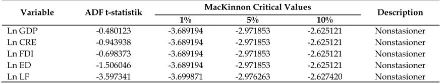
Unit root test is done one by one or all variables in the analysis that will be both dependent and independent variables. Unit root test results are obtained on the level, and it can be seen in table 2.
Table 2 shows that no variable is stationary either Gross Domestic Product (GDP), bank credit, Foreign Direct Investment (FDI), Foreign Debt or labor force at the level. This shows that the test data should continue with the degree of integration testing.
Integration Degree Test
Because the unit root test with observed data at level is not stationary, it is necessary to proceed with trials testing degree of integration. This test is intended to determine what degree of observed data is stationary. Because the degree of integration testing is a continuation of the unit root test, the test step is identical to the unit root test to distinguish difference in the course and assumptions used are the same hypothesis.
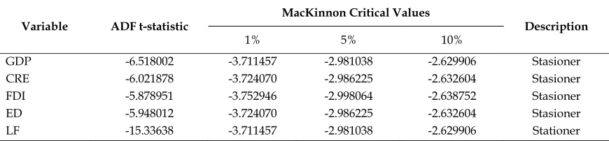
Table 3 shows the results of the unit root test on the 1st level difference which showed an improvement, but not all variables showed stationary. Still there is one variable that is AK (Labor Force) who have not stationary, it is necessary to continue testing the unit roots at 2nd level difference.
Table 4 (Appendix) showed that five variables have been stationary at the second
Table 2. Augmented Dickey Fuller Resultant Level
Variable ADF t-statistik MacKinnon Critical Values Description 1% 5% 10%
Ln GDP -0.480123 -3.689194 -2.971853 -2.625121 Nonstasioner
Ln CRE -0.943938 -3.689194 -2.971853 -2.625121 Nonstasioner
Ln FDI -0.698373 -3.689194 -2.971853 -2.625121 Nonstasioner
Ln ED -1.506046 -3.689194 -2.971853 -2.625121 Nonstasioner
level difference, the variable Y (GDP), CREDIT, FDI, Foreign Debt and AK, at a significance level of 5 percent. Therefore it can be said that all the data used in this study are integrated the second difference.
Long-Term Analysis
Cointegration Test. Cointegration test used in this study employed Engel and Granger method, by making the DF-AD F statistic test to see whether the co integration regression residuals is stationary or not. To calculate the value of the DF and ADF equation first cointegration regres-sion was formed by the method of ordinary least squares (OLS). Then after the regression equation residuals from the equation were obtained. Regression equation is formulated as follows:
Yt = β0 + β1LnFDIt + β2LnEDt + β3LnCREt +
β4LnLFt + et
The results of equation Engle-Granger cointegration test is as follows:
Yt = β0 + β1LnFDIt + β2LnEDt + β3LnCREt +
β4LnLFt
. . .
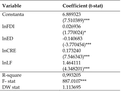
. .
Based on table 5 it can be seen that the whole of each independent variable (FDI, Foreign Debt, CRE, LF) significantly affects the dependent variable (GDP). FDI has positive coefficient (0.026936), with a probability value
of 0089 or significant at 10 percent level. These results are certainly consistent with the hypo-thesis that states that there is a positive effect between FDI and economic growth in the long run.
Table 5. The Result of Engle Granger cointegration test for long-term
Variable Coefficient (t-stat)
Constanta 6.889323
(7.510389)***
lnFDI 0.026936
(1.770024)*
lnED -0.140683 (-3.770454)***
lnCRE
lnLF
0.173240 (7.546343)*** 1.464111 (4.348201)***
R-square 0,993205
F- stat 887.0107***
DW stat 1.113695
( ) shows standard error; ***significance at level 1%; **significance at level 5%; *significance at level 10%
The results of this study demonstrate that in the long run there is a positive correlation between FDI growth rates in Indonesia. This is because high levels of FDI will increase pro-duction capacity, capability, which ultimately led to the opening of new jobs. Thus, the unem-ployment rate is reduced and the ordinary people's income will increase. The presence of FDI also allows the transfer of technology and knowledge from developed countries to devel-oping countries.
However, when seen from the regression coefficient, variable of FDI in the long-term relationship indicates that is relatively small numbers and the significance level is quite low. Table 3. Augmented Dickey Fuller result at 1st Difference
Variable ADF t-statistik MacKinnon Critical Values Description 1% 5% 10%
GDP -3.722986 -3.699871 -2.976263 -2.627420 Stasioner
CRE -4.249008 -3.699871 -2.976263 -2.627420 Stasioner
FDI -6.160319 -3.699871 -2.976263 -2.627420 Stasioner
ED -4.638136 -3.699871 -2.976263 -2.627420 Stasioner
This indicates that the contribution of FDI as a driving force of economic growth in Indonesia is still not optimal. This is because there are still many problems faced in their own country, such as upholding the rule of law, labor law, regional autonomy and other issues that have not created a conducive of investment climate.
Although the rate of investment in Indone-sia is still relatively minimal compared to countries in Southeast Asia and various invest-ment problems in Indonesia, but in fact the figure is still able to contribute to the devel-opment of Indonesia's GDP. This indicates that the multiplier effect of FDI is quite a positive impact on GDP growth. Foreign Debt have a negative coefficient (-0.140683), with a proba-bility value of 0.0009 or significant at 1 percent level. These results are certainly not consistent with the hypothesis that states that there is a positive effect between Foreign Debt and eco-nomic growth in the long run.
Although in theory there is positive effect of foreign debt to GDP, but based on the results of the analysis in the long run it turns negative effect on GDP as a result of several factors, including; there still a large amount of foreign debt from year to year as well as the large amount of debt principal repayments and inter-est to be paid by the government. Since the orde baru government to Indonesia bersatu govern-ment, one of the economic policies that never changes is the use of foreign debt as a source for the development cycle of the grant, which is always contained in the structure of the state budget (APBN). So it is not surprising that a buildup of foreign debt alone swelled from year to year. Every year, the government is obliged to pay the foreign debt. To pay the debt princi-pal repayments and interest, the government was forced to seek new debt which is never suf-ficient in amount to pay the debt on any of the current budget. If we look at the fact that Indo-nesia's foreign debt continues to increase from year to year and to reach 2000 trillion more in 2013, it can be said that in such circumstances the Indonesian nation has entered into a debt trap, which forced the government to "dig a hole close the holes " to pay the of foreign debt each year.
In addition to the low added value of debt as a source of funds for development, such as
foreign debt is not appropriate, make foreign debt negatively impacts the main objective of foreign debt capital increase that will have an impact on economic growth in Indonesia. Sev-eral studies have shown that the greater the debt of a country, the greater the potential for corruption and misuse of funds of the debt (Anwar, 2011).
Another factor is the cause of the increas-ing foreign debt but it is not a positive influence for Indonesia to borrow in dollars and the value of the rupiah against the dollar continues to fluctuate, so that the actual foreign debt increases but not the amount of the loan it is due to the increase in the exchange rate against the dollar. For example, when there is a crisis in 1998 foreign debt rose sharply to reach 573 tril-lion from the previous year amounted to 269 trillion, and the type we saw the rupiah against the dollar also raised sharply from 4650 in 1997 to 8025 in the next year, and continued to increase from year to year.
Bank credit has a positive coefficient (1.464111), with a probability value of 0:00 or significant at the 1 percent level. These results are certainly consistent with the hypothesis that states that there is a positive effect between bank credit and economic growth in the long run. These results are consistent with the theory of the relationship between bank credit and economic growth, which states that banks credit can create and boost business and employment field. Bank credit can create and improve the distribution of the community’s income. Indi-rect lending by the bank will increase state rev-enue from corporate taxes that are growing and developing its business volume (Herlina, 2011).
aggregate productivity increases, so it will ulti-mately have an impact on economic growth of a region (Soeparno, 2011).
The result of the estimation of the long-term equation shows the v alue of F-statistic 887.0107 with a probability value 0.00000. This value is smaller than 1 percent significance level so that it can be concluded that together there is significant influence between independent vari-ables as a whole is made up of Foreign Direct Investment (FDI), Foreign Debt, Bank Credit and Labor Force to variable dependent Gross Domestic Product.
The results of the estimation of the long-term equation show that the value of DW (Durbin Watson) was 1.113695. This shows the model does not contain autocorrelation because the DW value is between -2 to +2. After we did the test of ordinary least squares method (OLS) then we will have a residual variable, and then proceed to test the residual variable, whether stationary or non stationary. The result of data processing co integration test can be seen in Table 6.
Table 6 shows that the variable e has been stationary at the second difference level. This means there is an indication that the variable e
for the data second difference and the long lag 1 does not contain a unit root, in other words the variable e is already stationary, so it is con-cluded that there is co integration between all variables included in the model Y (GDP). This has the meaning that in the long run there will be a balance or stability between observed variables.
Short-Term Analysis
Error Correction Model (ECM) Tests. Having escaped from the cointegration test, the next step is to form the equation error correction model (ECM). The equation to be set up as follows:
∆ ∆ ∆
∆ ∆
∆
Description: Yt = Gross Domestic Product in period t; LnFDI = Foreign Direct Investment in period t. LnEDt = Foreign Debt in period t; LnLFt = Labor Force in period t; LnCREt = Bank lending period t; ECTt-1= error correction term in the previous period
The above equation is constructed based on the results of the test that all variables have been stationary in the second difference shown by the notation Δ. Error correction model (ECM) is used to estimate the short-term dynamic models of the variable gross domestic product. Use of ECM estimation methods can combine short-and long-term effects caused by fluctua-tions and time lags of each independent varia-ble. Based on the results of the ECM test showed the following results on table 7.
Table 7. Engle Granger Cointegration test result for short-term
Variable Coefficient (t-stat)
Constanta 0.042764 (1.894009)*
DFDI(-2) 0.026601 (2.209709)**
DED(-2) -0.140683 (-3.770454)***
DCRE(-2)
DLF(-2)
0.149893 (6.543326)*** 0.840824 (1.983408)**
E(-2) -0.604796
(-2.429299)**
R-square 0.827312
F- stat 20.12127*
DW stat 1.461093
( ) standard error; ***significance at level 1 %; **significance at level ; 5 %; *significance at level 10%
Tabel 6. Augmented Dickey Fuller result in residual equation
Variable ADF t-statistic MacKinnon Critical Value Result Description
1% 5% 10%
The equation above is a dynamic model of economic growth (GDP) for the short term, where the GDP variable is not only influenced by the Foreign Direct Investment (FDI), foreign debt, bank credit and the labor force but also influenced by variable error term et. Coefficient
et appears here significant value to be placed in the model as a short-term correction in order to achieve long-term balance. The smaller the value of et, the faster the process of correction to the long-term equilibrium.
Therefore, the ECM variable et is often said to be a factor as well as inaction, which has a value less than zero, et < 0. In this model, the value of the coefficient et reached -0.604796, which indicates that the value of the Gross Domestic Product (GDP) is above long-term value. So that needs to be corrected each year by -0.604796 to achieve long-term balance. ECT value or E (-2) -0.604796 significant at the 5 percent level indicates that the resulting model is valid.
The estimation results of the short-term equation shows R-Square value of 0.827312, meaning that 82.73 percent of the economic growth model can be explained by variable changes in FDI, foreign debt, bank credit and the labor force in the previous year period. While the rest of 17.27 percent is explained by other variables outside the model.
The results of the short-term equation show the value of the F - statistic is 20.12127 with a probability value 0.0. This value is smaller than 1 percent significance level so that it can be con-cluded that together there is significant influ-ence between independent variables as a whole is made up of foreign direct investment, foreign debt, bank credit and the labor force to the dependent variable gross domestic product.
Foreign Direct Investment (FDI) in the short-term have positive effect on economic growth and is symbolized by Gross Domestic Product (GDP) with a significance level of 5 percent with a coefficient of 0.026601. The result of this coefficient is almost the same as in the estimation of the long-term results, but has a higher level of significance. For the long-term estimate is only significant at the 10 percent level. This means that there is a tendency that FDI has more affect to economic growth in the short term. Foreign debt in the short-term has
a negative effect on economic growth sym-bolized by Gross Domestic Product (GDP) with a significance level of 1 percent with a coefficient -0.140683. The results of this coefficient are equal to the estimation results in the long run, both in the level of significance and coefficient. This means that both the long-term and short-term foreign debt has the same effect.
Bank credits in the short-term have a posi-tive effect on economic growth symbolized by the Gross Domestic Product (GDP) with a sig-nificance level of 1 percent with a coefficient 0.149893. The results of this coefficient are larger than the estimation results in the long term, but have the same significance level. This means that there is a tendency that bank credit more affects economic growth in the short term. The labor force in the short-term have a positive effect on economic growth symbolized by the Gross Domestic Product (GDP) with a signifi-cance level of 5 percent with a coefficient of 0.840824. The result of this coefficient is higher than estimated in the long term, but at the lower level of significance. This means that there is a tendency that the labor force has more have effects in the long-term over economic growth.
CONCLUSION
economic growth in Indonesia with 1.46 coeffi-cient significant at one percent level, while the short-term bank lending also has a positive effect on economic growth with a coefficient of 0.15 significant at the one percent level. This means that bank credit is more influential in the long term; 4) The labor force in the long-term has a positive effect on economic growth in Indonesia with a coefficient of 0.17 a significant at the one percent level. While in the short term there is also a positive effect on economic growth with a coefficient 0.84 and significantly decreased to 5 percent level. This means that there is a tendency that the labor force is more influential in the long run.
To be able to enhance the growth of invest-ment in Indonesia, the governinvest-ment should be able to seek a favorable investment climate, eco-nomic stability, improve the security of the state and the proper regulation so that investors, both foreign and domestic, can feel safe and keen to invest their capital so the result can increase economic growth. In terms of FDI, the government should be able to weigh the bene-fits of both short-term and long-term invest-ment by foreigners. As well as more selective in choosing foreign companies to invest in Indo-nesia that gives more benefit.
The development foreign debt must be considered in order to remain in the normal position and the favorable economic develop-ment does not increase the burden of the Indo-nesian economy. For long-term debt can be detrimental to the economy because the risk is greater. The need for reevaluation of debt is undertaken in order to provide benefits rather than to the detriment of the country. Indonesia's economy is still vulnerable to outside influ-ences, so the value of the exchange rate is still not stable to a great cause and should be con-sidered by the government in taking foreign debt. Using mudharabah and musyarakah skim (Profit loss sharing) to increase basis for eco-nomic development that will encourage the real sector, and in turn will reduce national depend-ence on foreign fund (Foreign debt and FDI).
Bank credit should be noted again until covers all the lines, so it can create a balanced distribution of capital between large and small.
So inequality of economic growth can be
avoided
. It is necessary to increase the laborproductivity through increased budgetary allo-cation to eduallo-cation in order to enhance the quality of the workforce, provide skills training for workers and expanding employment op-portunities so that output increases may ulti-mately spur economic growth in Indonesia.
REFERENCES
Anwar, Arwiny Fajriah. (2011). Analisis penga-ruh utang luar negeri dan penanaman modal asing terhadap produk domestik bruto di
Indonesia. Makassar: Fakultas Ekonomi
Universitas Hasanuddin
Diah, Indira. (2011). Dampak pembayaran utang luar negeri swasta pada penentuan nilai tukar dengan pendekatan moneter periode 2002-2009.
Jakarta: Fakultas Ekonomi UI.
Gujarati, Damodar. (1999). Ekonometrika Dasar. Jakarta: Erlangga.
Herlina, Siti Desimayanti. (2011). Analisis kredit perbankan pada bank umum konvensional. Jakarta: Fakultas Ekonomi, Universitas Gunadarma.
Kamaludin, Rustian. (2007). Beberapa aspek pem-bangunan perekonomian daerah dan hubungan keuangan luar negeri. Edisi kedua. Jakarta: UniversitasTrisakti.
Liwan, Audrey dan Evan Lau. (2007). Managing growth: The role of export, inflation and invest-ment in three ASEAN neighboring countries.
Munich Personal RePEc Archive, Malaysia. Mardalena, Ervin. (2009). Pengaruh investasi
swasta dan perdagangan internasional terhadap pertumbuhan ekonomi di Suma-tera Selatan. JurnalEkonomika.
Nachrowi, D. Nachrowi. (2006). Ekonometrika, untuk analisis ekonomi dan keuangan. Cetak-an pertama. Jakarta: Lembaga Penerbit FE UI.
Soeparno. (2011). Analisis indikator makroekonomi terhadap pertumbuhan ekonomi. Medan: Fa-kultas Ekonomi Universitas Sumatera Utara.
Syaharani, Febrina Rizki. (2011). Pengaruh pe-nanaman modal dalam negeri, pepe-nanaman modal asing, dan utang luar negeri terhadap pertumbuhan ekonomi Indonesia 1985-2009.
Jakarta: Fakultas Ekonomi dan Bisnis Universitas Islam Negeri Syarif Hida-yatullah.
Tambunan, Tulus. (2007). Daya saing Indonesia dalam menarik investasi asing. Jakarta: Bank Indonesia.
Thomas, R.L. (1997). Modern econometrics: An introduction. Harlow: Addison-Wesley. Todaro, Michael P. (2000). Pembangunan ekonomi
di dunia ketiga 2, alih bahasa oleh Haris Minandar. Jakarta: Penerbit Erlangga. Utari, G.A Diah, Trinil Arimurti, Ina Nurmalia
Kurniati. (2012). Optimal credit growth.
Buletin Ekonomi Moneter dan Perbankan.
Oktober 2012. www.bps.go.id www.bi.go.id www.bkpm.go.id
APPENDIX
Table 4. Augmented Dickey Fuller result at2nd Difference
Variable ADF t-statistic
MacKinnon Critical Values
Description
1% 5% 10%
GDP -6.518002 -3.711457 -2.981038 -2.629906 Stasioner
CRE -6.021878 -3.724070 -2.986225 -2.632604 Stasioner
FDI -5.878951 -3.752946 -2.998064 -2.638752 Stasioner
ED -5.948012 -3.724070 -2.986225 -2.632604 Stasioner