How Disasters Affect Local Labor
Markets
The Effects of Hurricanes in Florida
Ariel R. Belasen
Solomon W. Polachek
a b s t r a c t
This study improves upon the Difference in Difference approach by examining exogenous shocks using a Generalized Difference in Difference (GDD) technique that identifies economic effects of hurricanes. Based on the Quarterly Census of Employment and Wages data, worker earnings in Florida counties hit by a hurricane increase up to 4 percent, whereas earnings in neighboring counties decrease. Over time, workers experience faster earnings and slower employment growth than workers in unaffected counties. Hurricanes have a greater impact in coastal and Panhandle counties, and powerful hurricanes have greater economic effects than weaker ones. Further, the GDD technique is applicable to analyze a wider range of exogenous shocks than hurricanes.
I. Introduction
An exogenous shock is an unexpected event that impacts a given market. Such shocks can take many forms, ranging from unexpected new legislation, to sudden population shifts, to domestic weather-related events, and even to terrorist attacks. A number of studies utilize Difference-in-Difference (DD) estimation to ex-amine the effects of exogenous shocks. For example, Card (1990) in a well-cited ar-ticle used DD to examine migration and found relatively small effects on wages. Such studies look at changes across time periods between the region of interest and a comparable region which was unaffected by the shock to find long-run effects. Angrist and Krueger (1999) call these results into question for failing to identify an
Ariel R. Belasen is an assistant professor of economics and finance at Southern Illinois University in Edwardsville, Ill. Solomon W. Polachek is a distinguished professor of economics at the State University of New York at Binghamton. All data contained in this paper will be made available upon request. The authors would like to thank Joel Elvery, Christopher Hanes, Kajal Lahiri, and Stan Masters along with the seminar participants at: SUNY Albany; SUNY Binghamton; the Third Migrant IZA Conference, Washington, D.C. March 2007; and the Twelfth Society of Labor Economists Meetings, Chicago, May 2007 for their comments.
½Submitted July 2006; accepted September 2007
ISSN 022 166X E ISSN 1548 8004Ó2009 by the Board of Regents of the University of Wisconsin System
appropriate control group. Perhaps, as a result, there is now a literature on appropri-ately choosing control groups, for example Bertrand, Duflo, and Mullainathan (2002), Kubik and Moran (2003), and Abadie, Diamond, and Hainvellen (2007). An-other problem is the experimental group. Most papers examining exogenous shocks rely on one experimental group; in Card’s (1990) case, this experimental group is Miami, the site of the Mariel Boatlift. However it is not obvious that one experimen-tal group suffices. In the Card example, the Miami labor market might not be typical of other potential experimental sites. Perhaps in his study, Miami’s unemployment did not rise because Miami’s economy was growing more rapidly than other simi-larly sized cities. This paper finds that by properly addressing these two issues, one can better isolate the direct impact of exogenous shocks. We find that counties hit by hurricanes experience a positive net effect on earnings and a negative net effect on employment, but that these effects dissipate over time.
One innovation of this paper is to havemanyrandom experimental groups as well
asmanyrandom control sites. To achieve this, we use a different natural experiment,
hurricanes, to examine the effect of an exogenous shock on a local labor market. Hurricanes, in particular, are a good choice for this study because they can affect sev-eral counties at a time, and can occur more than once in the time period under study. By having many experiment sites, we are able to test how the impact of exogenous shocks differs by both characteristics of the shock and characteristics of the experi-ment group. Other papers have used weather-related events such as rainfall (includ-ing Miguel 2005; Waldman, Nicholson, and Adilov 2006; and Connolly 2007) to obtain a purely exogenous variable as an instrument to predict other independent var-iables such as how much television children watch (in the case of Waldman et al. 2006), which in turn is used to predict autism using a simultaneous equation
ap-proach. We use weather (that is hurricanes) directly astheexogenous shock we want
to evaluate.
To do this, we develop a Generalized Difference-in-Difference (GDD) technique in which we compare affected regions to unaffected regions across multiple exoge-nous events and time periods. In addition, exogeexoge-nous shocks that are felt positively by one specific labor market can also have an effect on nearby labor markets. Thus we can examine multiple exogenous shocks affecting more than one locality at a time. Further, to address the issue of the appropriate definition of treatment and con-trol groups, we compare a given hurricane-stricken county to all other unaffected counties within that state. In addition, by using quarterly time-series data, this ap-proach has the advantage of distinguishing short-term and long-term effects that pre-viously had been neglected. In this way we can better identify the effect of an exogenous shock as well as quantify its effect over time.
The destructive power of hurricanes worldwide can wipe out thousands of lives and cause billions of dollars worth of infrastructure and private property losses
an-nually. Hurricane season runs from June 1stthrough November 30theach year over
warm water, defined as oceanic temperatures exceeding 80 degrees Fahrenheit. How-ever, the exact timing and path of the hurricanes cannot be determined in advance. Due to the high temperatures required, most hurricanes that strike the United States strike the Gulf States and the Southeastern States. Because Florida is a member of both subsets of states, it is instructive to look at the county-level Florida labor market to examine the exogenous shocks of hurricanes.
Over the course of an average year, the state of Florida will generally see one to two hurricanes during the six-month hurricane season, but there are years when Flor-ida is not hit, even once. Over the last two years of the sample (2004 and 2005), how-ever, the hurricanes that struck Florida were more frequent and more powerful than
ever before.1Although hurricanes are not completely unexpected shocks to the state
of Florida, each hurricane event is exogenous to the specific counties that are hit as well as to the degree of damage unleashed. Therefore, the events we have identified can be used as an independent variable by comparing those counties that have been hit to the other counties that avoided devastation.
Florida is comprised of 67 counties and, over the past 18 years, none of them have escaped the effects of hurricanes. Five of the six most damaging Atlantic hurricanes of all time have struck Florida over the course of this time period. Damages to prop-erty can be estimated in direct monetary costs, for example, 1992’s Hurricane Andrew wound up costing Southern Florida roughly $25.5 billion ($43 billion in 2005 USD) in property losses (Rappaport 1993). However, a county, business or per-son’s wealth is made up of more than just the stock of assets owned by that person. A major portion of the flow of one’s wealth comes from earned income. Thus the ques-tion is raised, how can the income-specific and employment-specific effects of a hur-ricane be measured? In addition, when looking at the effects of a hurhur-ricane on a specific county, are there any spillovers that need to be accounted for in neighboring counties? In addition, do more destructive hurricanes impact labor markets more intensely? And finally, how long are the effects of a hurricane felt in earnings and employment?
II. Background on Florida and
the Hurricanes
Over the course of the last 18 years, the state of Florida has been rav-aged by 19 hurricanes. A summary table containing descriptive statistics for each of the hurricanes can be seen in Table 1, which lists magnitude, monetary costs, and death statistics for each storm. Each hurricane is given a standard name by the World Meteorological Organization assigned to the storm in alphabetical order each year based on the timing of the storm. The lists of names for hurricanes change each year, with the gender of the initial storm also alternating each year. There are six lists in total and any time a particularly devastating hurricane occurs, the name of that hur-ricane is ‘‘retired’’ from the list (Padgett, Beven, and Free 2004). After the sixth list is used, the first is then cycled back with any retired hurricane names replaced with new names beginning with the same letter as the retired ones.
1. The National Oceanic and Atmospheric Administration retires the names of particularly devastating hur-ricanes. Nine of the nineteen hurricanes in the sample occurred in the 2004 and 2005 hurricane seasons. Eight of those storms have had their names retired (as opposed to just three retirees throughout the remain-der of the sample), including Hurricane Wilma which set records for intensity. Note, however, that in this past 2006 season, Florida was only hit by one minor hurricane: Ernesto, so this is not necessarily a trend moving forward.
Table 1
Descriptive Statistics
Hurricane
Synoptic Lifecycle
Damage to Florida
Deaths in Florida
Windspeed at Landfall
Average Rainfall
Saffir Simpson Scale
Florence September 1988 $0.6 million 0 75 mph 5"–10" 1
Andrew August 1992 $43 billion 44 175 mph 5"–7" 5
Allison June 1995 $1.2 million 0 75 mph 4"–6" 1
Erin August 1995 $0.5 million 6 87 mph 5"–12" 1
Opal September 1995 $4.4 billion 1 115 mph 5"–10" 3
Danny July 1997 $100 million total to U.S. 0 80 mph 2"–7" 1
Earl September 1998 $64.5 million 2 92 mph 6"–16" 1
Georges September 1998 $392 million 0 103 mph 8"–25" 2
Irene October 1999 $1.1 billion 8 75 mph 10"–20" 1
Gordon September 2000 $11.9 million 1 75 mph 3"–5" 1
Charley August 2004 $15.1 billion 29 150 mph 5"–8" 4 Frances September 2004 $8.9 billion 37 105 mph 10"–20" 2
Ivan September 2004 $8.1 billion 19 130 mph 7"–15" 3
Jeanne September 2004 $6.9 billion total to U.S. 3 121 mph 8"–13" 3 Dennis July 2005 $2.2 billion 14 120 mph 10"–15" 3 Katrina August 2005 $115 billion total to US 14 81 mph 5"–15" 1 Ophelia September 2005 $70 million total to US 1 80 mph 3"–5" 1 Rita September 2005 $10 billion total to US 2 80 mph 2"–4" 1 Wilma October 2005 $12.2 billion 35 120 mph 7"–12" 3
Source: National Oceanic and Atmospheric Administration
Note: Retired Hurricanes areitalicized; all damage is to Florida unless otherwise noted.
254
The
Journal
of
Human
Hurricanes are categorized according to the Saffir-Simpson Scale based on their wind speed. Hurricanes Florence, Allison, Erin, Danny, Earl, Irene, Gordon, Ophelia, and even the Floridian part of Katrina were Category 1 hurricanes at landfall, mean-ing they had wind speeds rangmean-ing between 74 and 95 miles per hour. Hurricanes Georges, Frances, and Rita were Category 2 hurricanes and had wind speeds ranging between 96 and 110 miles per hour. With wind speeds ranging between 111 and 130 miles per hour, Hurricanes Opal, Ivan, Jeanne, and Dennis were classified as Cate-gory 3 hurricanes. Hurricane Charley reached 150 miles per hour and became Cat-egory 4 as it hit the mainland. Hurricanes Andrew and Wilma were CatCat-egory 5 hurricanes and had winds well above 180 miles per hour.
III. Economic Model of Hurricanes
According to Lucas and Rapping (1969), when people perceive a shock as having a temporary effect on the economy, they will not alter their long term perception of the economic variables that are affected by the shock. Hurricanes generally last for, at most, two or three days once they strike land. Historically speak-ing, even the damages from the most destructive hurricanes are typically repaired within two years of the hurricane. Therefore, one would expect to see perceptions of the future remain largely unchanged in the long run as the variables return to their steady state levels of growth. Guimaraes, Hefner, and Woodward (1993) state that while hurricanes create an economic disturbance in the short run, oftentimes they can lead to economic gains in the long run.
More specifically, within labor demand and labor supply, hurricanes will lead to negative shocks on labor supply in the stricken region, along with undetermined shocks to the region’s labor demand as some firms attempt to fill vacancies in their work force while others leave town with the outflow of workers. If a hurricane strikes a region and causes people to flee, the work force in that region will decrease. There-fore, labor supply would shift downward. At the same time, if that hurricane destroys a lot of private property and physical capital, labor demand could also decrease as employers have to close their shops. However, Skidmore and Toya (2002) point out that the risk of a natural disaster can reduce the expected return to physical cap-ital (which may be destroyed during the storm) and, in turn, there is a substitution effect toward human capital as a replacement. Of course, as the demand for human capital rises, the price of human capital will also rise. This leads to an income effect that runs counter to the substitution effect. On the other hand, if the hurricane only destroys residential areas, labor demand also could increase as employers attempt to fill vacant jobs. Thus, the shock on labor demand from a hurricane most likely will be positive leading to changes in earnings and employment.
Using the standard labor market framework, with labor supply shocked negatively and labor demand shocked positively, earnings will increase, and employment will have an ambiguous effect depending on whether or not the demand shock outweighs the supply shock. The set of earnings and employment that we are examining in this study are county-level average quarterly earnings per worker in the state of Florida. In order to measure the actual earnings effects of hurricanes on earnings, we will control for other factors that have an effect on earnings and employment. Florida’s
economy has been growing rapidly over the last half-century and every county in Florida has benefited from this growth. Card (1990) found that immigrants in Miami had no long-term effects on wages despite increasing the labor force by 7 percent. He deduces that the Florida labor market in the 1980s was able to simply absorb a group of 45,000 immigrants into the labor market without a change in wages because of the rapid growth of Florida’s economy. Ewing and Kruse (2005) isolated the specific county-level fluctuations from the overall general growth by controlling for the trend of earnings movement across the entire state. In a subsequent paper, Ewing, Kruse, and Thompson (2007) explained that local economies may be influenced by state business cycles. Following their method, we control for the state trends of Florida. Furthermore, Florida’s labor market is greatly influenced by seasonal shifts. During the summer months, earnings and employment decrease in several sectors of the la-bor market. Thus, one must also control for seasonality.
In the end, we have two equations, one for employment (Qit) and one for earnings
(yit) which sets the dependent variable equal to a function of state (Qt,yt), county-spe-cific time-invariant effects (Zi), seasonal trends (St) as well as hurricane effects (Hit):
Qit ¼fðQt;Zi;St;HitÞ+uit
ð1Þ
yit¼fðyt;Zi;St;HitÞ+vit
ð2Þ
As stated earlier, an important question to consider when examining hurricanes and other exogenous shocks is what kind of neighboring effects, if any, will affect the model. If a hurricane forces workers to flee one county for a second county, then labor supply in the original county will be negatively affected while labor supply in the second county will be positively affected. Thus, the model is set up to include a series of hurricane dummy variables that capture direct effects and neighboring effects. This allows us to compare three distinct sets of counties: those that were di-rectly hit and faced heavy destruction, those that were close by, and thus affected by heavy rainfall, and those that were farther out, and generally unaffected by the
hur-ricane. Assuming that countiesiandjborder one another, the subscriptiunderHD
indicates that the locus of destruction2 from the hurricane is directly passing over
countyiwhile subscriptijunderHNindicates that the locus of destruction of a
hur-ricane is passing through countyjwhich borders countyi. In other words,HDtakes a
value of one when the hurricane strikes countyi; andHNtakes a value of one when
the hurricane strikes countyjbut not countyi. More specifically,
Qit ¼u1iQt+u2iZi+u3iZit+u4iSt+u5iHDit +u6iHijtN +uit
ð3Þ
yit¼f1iyt+f2iZi+f3iZit+f4iSt+f5iHDit +f6iHNijt+vit
ð4Þ
Since the immediate effects of hurricanes are felt in a matter of days, we will first-difference the equations to examine the changes of average quarterly earnings per worker rather than strictly looking at the levels of quarterly earnings per worker; and the changes in employment rather than the level of employment. That way we
2. The locus of destruction is defined to be the area directly around the eye of the hurricane in which the radar measurements of the storm exceed 40 dBZ. For a typical hurricane, the ring’s radius can measure out between 20 and 30 kilometers.
can eliminate any time-invariant county-specific effects. In addition, we also exam-ine the change in the growth rates of employment and earnings from one period to the next, by naturally logging each equation and rewriting them in first-difference notation:
Due to space limitations, we only present the results emanating from Equations 6 and 8. Results emanating from the other equations are available upon request.
IV. Application of the Model
Theoretically, employment in the average Florida county should in-crease by the same percentage as employment in Florida as a whole inin-creases. With
such uniform growth, the coefficient for state employmentðu1iÞ should be positive
and equal to one whenQtis defined as average county employment. Thus we
mea-sureQtas state employment in timetdivided by 67 (the number of Florida counties).
Similarly, uniform growth impliesf1iin (8) should be one whenytis defined as
earn-ings per worker. The summer seasonal trend appears to strictly impact the labor sup-ply function by increasing employment and thus decreasing earnings, so we expect to
seeu4i.0 andf4i,0. Economic theory predicting that labor supply and labor
de-mand offset each other with regards to employment, and/or that labor dede-mand is
highly inelastic implies thatu5i,0 andu6i.0. Finally, since hurricanes negatively
affect labor supply in the county that gets hit and positively affect labor supply in
nearby counties as workers relocate,f5ishould be positive andf6ishould be
nega-tive as the equilibrium wage adjusts to the change in employment. And because workers from the same stricken county may flee to several different counties, the
magnitude off5ishould be greater than that off6ibecause the impact on a directly
hit county will likely be greater than on a county that was nearby a hurricane. The hurricane data used in this analysis come from the National Hurricane Center
of the National Oceanic and Atmospheric Administration (NOAA).3The NOAA is a
federal agency within the Department of Commerce that examines the conditions of the oceans and the atmosphere. In particular, the NOAA evaluates ecosystems, cli-matic changes, weather and water cycles, and commerce and transportation. The Pew Center on Global Climate Change (2006) reports that the strength and frequency of hurricanes have increased to unprecedented levels over the past decade. In the last few years specifically we have seen hurricanes appear in places like the South Atlan-tic that had previously been thought of as safe from hurricanes. One such storm
3. National Oceanic and Atmospheric Administration, http://www.noaa.gov/
struck Brazil in March 2004 and wreaked havoc along the coastline because people had not had any experience dealing with hurricanes (Climate.org 2004). Even Flor-ida, with its high rate of storms each year, has had difficulty dealing with the higher frequency and higher magnitude storms in the past few years. Therefore, to balance the high intensity of the last decade we are also including hurricanes that struck Flor-ida in the decade prior to this one. All in all, 19 hurricanes of varying strength struck Florida in the 18-year period between 1988 and 2005.
To coincide with this time period, quarterly employment4and average quarterly
earnings data from the Bureau of Labor Statistics (BLS) Quarterly Census of
Em-ployment and Wages (QCEW)5 were used, spanning the time period starting with
the first quarter of 1988 and continuing through the fourth quarter of 2005.6 The
BLS surveys employers regarding their total wage bill and employment each quarter. The employers are sorted by county, such that each report of employment is recorded for the county in which the workers are employed.
The regression can be run using a GDD procedure which is similar to a DD ap-proach taken over multiple events and time periods to compare the effects of hurri-canes on Florida’s counties. The process estimates the difference between the first differenced fixed-effects transformation to calculate the impact of hurricanes by comparing the counties that were hit to those counties that were not hit, and con-glomerate the coefficients across counties, thereby eliminating the county-specific coefficients. Thus, we force the coefficient on the state trend to be equal to one by
bringing DlnQt andDlnyt to the left-hand side of the regression, and then relabel
the coefficients sequentially for ease of comparison:
ðDlnQit2DlnQtÞ ¼a1Zi+a2DSt+a3DHitD+a4DH
The dependent variables now measure the degree a county’s per-worker wage and a country’s employment deviate from the average Florida county.
As mentioned before, a value of one forDHD
itimplies that a hurricane passed right
through countyiat timet. A value of one forDHN
ijt implies that a hurricane did not
strike countyi, but instead struck a county that neighbors countyi. In that way, any
indirect neighboring effect from a hurricane will be captured in the data. We used the detailed magnitudes and coordinates from the NOAA to trace the path of destruction
that the hurricanes left behind as they passed through Florida.7At this point we
as-sume that all time-invariant county-specific effects will have no effect on growth, and
thus theZiterms will take values of zero. This assumption is relaxed in the next
sec-tion where we explore geographic differences. The results are captured in the first model of Tables 2 and 3.
4. Some employment data were available in a monthly format as well, and whenever possible, monthly data were used for employment.
5. Bureau of Labor Statistics, http://www.bls.gov/
6. Hourly employment data would be preferable for this study, however, due to data limitations, total em-ployment numbers were used instead.
7. To trace the path, we used Google Earth (2006) software package available for download at http://earth. google.com/.
Table 2
GDD Regression Results on Change in Growth of Employment in a Hurricane-Stricken County Relative to an Average County
Independent Variables Model 1 Model 2 Model 3 Model 4 Model 5 Model 6 Model 7 Model 8 Model 9 Model 10 Model 11
Summer Seasonal Effect
Coefficient: 0.0163*** 0.0152*** 0.0162*** 0.0165*** 0.0162*** 0.0164*** 0.0166*** 0.0163*** 0.0163*** 0.0164*** 0.0163***
P-value: 0.000 0.000 0.000 0.000 0.000 0.000 0.000 0.000 0.000 0.000 0.000
Direct Effect of Hurricanes
Coefficient: 20.0237*** 20.0149** 20.0132** 20.0115 20.0129** 20.0242*** 20.0301*** 20.0235*** 20.0440*** 20.0316*** 20.0702***
P-value: 0.000 0.019 0.047 0.121 0.038 0.000 0.000 0.000 0.000 0.000 0.001
Neighboring Effect of Hurricanes
Coefficient: 0.0024 0.0175** 0.0042 0.0013 0.0034 0.0017 20.0001 0.0036 0.0015 0.0002 0.0171*
P-value: 0.594 0.045 0.482 0.844 0.528 0.721 0.990 0.429 0.832 0.979 0.096
Interaction of Direct and Multiple
Coefficient: 20.0133
P-value: 0.203
Interaction of Neighboring and Multiple
Coefficient 20.0022
P-value: 0.838
Interaction of Direct and Death Toll
Coefficient: 20.0004
P-value: 0.227
Interaction of Neighboring and Death Toll
Coefficient: 0.0003
P-value: 0.396
Interaction of Direct and Retired
Coefficient: 20.0111
P-value: 0.411
(continued)
Belasen
and
Polachek
Table 2 (continued)
Independent Variables Model 1 Model 2 Model 3 Model 4 Model 5 Model 6 Model 7 Model 8 Model 9 Model 10 Model 11
Interaction of Neighboring and Retired
Coefficient: 0.0217
P-value: 0.116
Interaction of Direct and Damage
Coefficient: 20.0011
P-value: 0.104
Interaction of Neighboring and Damage
Coefficient: 0.0004
P-value: 0.525
Interaction of Direct and Election
Coefficient: 0.0046
P-value: 0.798
Interaction of Neighboring and Election
Coefficient: 0.0054
P-value: 0.708
Interaction of Direct and Early
Coefficient: 0.0308***
P-value: 0.005
Interaction of Neighboring and Early
Coefficient: 0.0320***
P-value: 0.010
Second County Away Effect
Coefficient: 20.0081
P-value: 0.152
Interaction of Direct and Coastal
Coefficient: 0.0348*** 0.0636***
260
The
Journal
of
Human
P-value: 0.001 0.000
Interaction of Neighboring and Coastal
Coefficient: 0.0019 20.0222*
P-value: 0.835 0.077
Interaction of Direct and Panhandle
Coefficient: 0.0265** 0.0749***
P-value: 0.012 0.000
Interaction of Neighboring and Panhandle
Coefficient: 0.0069 20.0223
P-value: 0.442 0.129
Interaction of Direct and C-P
Coefficient: 20.0813***
P-value: 0.000
Interaction of Neighboring and C-P
Coefficient: 0.0433**
P-value: 0.019
R2 0.0221 0.0268 0.0233 0.0237 0.0238 0.0222 0.0260 0.0226 0.0249 0.0238 0.0299
F 35.35 21.46 18.62 18.95 19.05 17.74 20.88 27.03 23.97 22.84 16.04
n, groups 4757, 67 4757, 67 4757, 67 4757, 67 4757, 67 4757, 67 4757, 67 4757, 67 4757, 67 4757, 67 4757, 67
Note: Table reports selected coefficients of equations (9, 11, 15, 17, and 19) fit with QCEW data. See text for details.
Included but not reported variables are the stand-alone dummy variables for each equation that correspond to each interaction term. *Significant at the 10% level; **Significant at the 5% level; ***Significant at the 1% level.
Belasen
and
Polachek
Table 3
GDD Regression Results on Change in Growth of Earnings Per Worker in a Hurricane-Stricken County
Independent Variables Model 1 Model 2 Model 3 Model 4 Model 5 Model 6 Model 7 Model 8 Model 9 Model 10 Model 11
Summer Seasonal Effect
Coefficient: 20.0283*** 20.0300*** 20.284*** 20.0283*** 20.0284*** 20.0283*** 20.0282*** 20.0282*** 20.0284*** 20.0284*** 20.0285***
P-value: 0.000 0.000 0.000 0.000 0.000 0.000 0.000 0.000 0.000 0.000 0.000
Direct Effect of Hurricanes
Coefficient: 0.0192*** 0.0055 0.0066 0.0176** 0.0095 0.0198*** 0.0262*** 0.0192*** 0.0208*** 0.0223*** 0.0206**
P-value: 0.000 0.364 0.303 0.013 0.111 0.000 0.000 0.000 0.005 0.000 0.027
Neighboring Effect of Hurricanes
Coefficient: 20.0093** 20.0282*** 20.0105* 20.0132** 20.0129** 20.0084* 20.0096** 20.0087** 20.0247*** 0.0041 20.009
P-value: 0.033 0.001 0.072 0.034 0.014 0.069 0.044 0.049 0.000 0.469 0.930
Interaction of Direct and Multiple
Coefficient: 0.0250**
P-value: 0.012
Interaction of Neighboring and Multiple
Coefficient: 0.0022
P-value: 0.835
Interaction of Direct and Death Toll
Coefficient: 0.0006*
P-value: 0.070
Interaction of Neighboring and Death Toll
Coefficient: 20.0004
P-value: 0.312
Interaction of Direct and Retired
Coefficient: 0.0066
P-value: 0.614
Interaction of Neighboring and Retired
Coefficient: 0.0140
P-value: 0.292
262
The
Journal
of
Human
Interaction of Direct and Damage
Coefficient: 0.0007
P-value: 0.256
Interaction of Neighboring and Damage
Coefficient: 20.0001
P-value: 0.921
Interaction of Direct and Election
Coefficient: 20.0047
P-value: 0.784
Interaction of Neighboring and Election
Coefficient: 20.0063
P-value: 0.650
Interaction of Direct and Early
Coefficient: 20.0198*
P-value: 0.060
Interaction of Neighboring and Early
Coefficient: 20.0062
P-value: 0.601
Second County Away Effect
Coefficient: 20.0046
P-value: 0.403
Interaction of Direct and Coastal
Coefficient: 20.0017 0.0038
P-value: 0.860 0.752
Interaction of Neighboring and Coastal
Coefficient: 0.0246*** 0.0079
P-value: 0.005 0.511
Interaction of Direct and Panhandle
Coefficient: 20.0167* 20.0204
P-value: 0.100 0.204
(continued)
Belasen
and
Polachek
Table 3 (continued)
Independent Variables Model 1 Model 2 Model 3 Model 4 Model 5 Model 6 Model 7 Model 8 Model 9 Model 10 Model 11
Interaction of Neighboring and Panhandle
Coefficient: 20.0321*** 20.0531***
P-value: 0.000 0.000
Interaction of Direct and C-P
Coefficient: 0.0024
P-value: 0.908
Interaction of Neighboring and C-P
Coefficient: .0356**
P-value: 0.046
R2 0.1467 0.1544 0.1483 0.1469 0.1481 0.1468 0.1478 0.1468 0.1482 0.1503 0.1526
F 267.9 142.26 135.58 134.1 135.4 134 135.09 201.08 162.58 165.38 93.42
n, groups 4746, 67 4746, 67 4746, 67 4746, 67 4746, 67 4746, 67 4746, 67 4746, 67 4746, 67 4746, 67 4746, 67
Note: Table reports selected coefficients of equations (10, 12, 16, 18, and 20) fit with QCEW data. See text for details.
Included but not reported variables are the stand-alone dummy variables for each equation that correspond to each interaction term. *Significant at the 10% level; **Significant at the 5% level; ***Significant at the 1% level.
264
The
Journal
of
Human
The coefficients that are of interest to this study area3;a4;d3, andd4, which re-spectively, are the direct and neighboring effects coefficients of hurricanes for each
of the four equations. In employment Equation 9,a3should reflect the average
per-cent deviation in employment growth between a county hit by a hurricane and one
not hit. Likewise,a4should represent the average percent deviation in employment
growth between a county bordering a county hit by a hurricane and an average Flor-ida county. We see that the number of workers falls by an average of 2.37 percent in counties that are struck directly by hurricanes relative to other counties (see Model 1
in Table 2).8The effect on neighboring counties is statistically insignificant, thus they
do not incur a noticeable change in the size of their employment.
The coefficients for the earnings function, Equation 10, can be interpreted as the average change in the growth rate of earnings per worker relative to the typical county. One can see from the results in Table 3 that the growth rate of earnings will change significantly in each of these two county types, with the directly hit counties’ growth rates of earnings increasing by 1.92 percent on average in the quarter that the
hurricane hits countyi(see Model 1 in Table 3). Similarly, the estimate ford4
indi-cates that the growth rate of earnings will fall by 0.93 percent on average in the
quar-ter in which a hurricane strikes a county that is neighboring countyi.
The underlying intuition behind these changes is that in directly hit counties labor supply will shift inward after a hurricane, thus leading to a decrease in employment and a subsequent increase in earnings. Within the neighboring counties where resi-dents will experience lighter flood damage, it appears that earnings fall despite no overall increase in employment. Belasen and Polachek (2008) show that this pattern is due to a change in the sectoral structure of the labor market in these counties. High-wage earners that are able to flee to safer regions will do so, leaving the low wage earners in their wake. Finally, as expected, the seasonal variables in the em-ployment equation are significantly positive for the change in emem-ployment and neg-ative for the employment equations which accounts for the summer trend in the state of Florida.
A significant source of error in this study lies with workers who do not work in the county they reside in. While most workers prefer to work near their homes, there will be a significant portion of the work force that travels a long distance to and from work each day. Additionally, if a county is declared a disaster zone, oftentimes relief workers are brought in from out of state and are not considered to be employed in the county they are assisting. We assume that these outliers are evenly distributed across the state labor market and thus should not affect any single county more than any other.9
A. Intensity Effects
Noting that the direct effects of hurricanes lead to increases in earnings, while neigh-boring effects lead to decreases in earnings, the question can be raised: Are the earn-ings effects similar across all hurricanes individually or are they more pronounced
8. This value is computed by comparing the additional change in employment incurred by the average hur-ricane-stricken county relative to the average unaffected county across the quarter in which a hurricane hit. 9. According to Joel Elvery of the BLS, the QCEW attempts to get accurate data on the relief workers via the source of their employment.
when a combination strike a county within the same time period? Equations 11 and
12 add in a dummy variable (M) to represent the presence of multiple hurricanes.
Multiple hurricane events are separated from individual hurricanes by including an
interaction term between the hurricane effect and theMdummy:
ðDlnQit2DlnQtÞ ¼a1DSt+a2DHitD+a3DHNijt
M, is interacted withDHDandDHNso that when a multitude of hurricanes strike a
county in Florida,Mwill take a value equal to one. The derivative of the difference in
employment growth with respect toDHDwill equal (a2+a5), and it will equal (a3+
a6) when taken with respect to DH
N. The derivative of the difference in earnings
growth with respect toDHDwill equal (d2+d5), and it will equal (d3+ d6) when
taken with respect toDHN. The interpretation of each of these derivatives is the
dif-ference in the growth rate of employment (or earnings) between the average
hurri-cane afflicted county and the overall average county. More specifically, a5 andd5
reflect the additional effect on employment and earnings resulting when multiple hurricanes strike a single county within the same quarter. One would suspect that a multitude of hurricanes will be much more destructive than a single hurricane and thus lead to much more capital loss and potential dispersion of the labor force, and therefore should have greater affects on labor demand and labor supply. The
results of the regression can be found in Tables 2 and 3 under Model 2.10
The coefficient for the interaction term ofMwith the direct effect in the
employ-ment equation reveals no additional effect on employemploy-ment growth resulting from multiple hurricanes beyond the effect of the initial hurricane. On the other hand, we find a significant effect for earnings. When multiple hurricanes directly strike a county, the relative growth rate of earnings in that county will rise by 2.5 percent on average. Note, however, that this increase replaces the standard direct effect
which is now insignificant.11Neighboring counties do not face any additional effects
resulting from a multitude of hurricanes.
Additionally, we also split up the hurricanes into two subcategories based on the Saffir-Simpson Scale. Hurricanes which fell into Categories 1, 2, or 3 made up the low-intensity group (SS1), and hurricanes in Categories 4 or 5 were placed into the high-intensity group (SS2). The group variables now replace the hurricane
vari-ables from the initial model. Thus the model takes the following form, whereSS1 and
SS2 correspond to the two Saffir-Simpson groups:
10. To conserve space, we do not reporta4andd4, or other ‘‘stand alone’’ dummy variables that
corre-spond to other interaction models described later in the text.
11. Models 3, 4, and 5 in Tables 2 and 3 employ alternative measures of hurricane intensity using a similar format as the multiple hurricane equations. Model 3 examines the impact of hurricane death tolls; Model 4 differentiates between hurricanes whose names have been retired from other hurricanes; and Model 5 exam-ines the monetary damage (in billions of 2005 dollars) to the State of Florida from each hurricane. (While county-level data would be more desirable, data limitations forced us to use state-level damage data.) In each instance, the effects were minor, if at all significant.
ðDlnQit2DlnQtÞ ¼a1DSt+a21DSS1Dit +a22SS2Dit +a31DSS1Nijt+a32DSS2Nijt
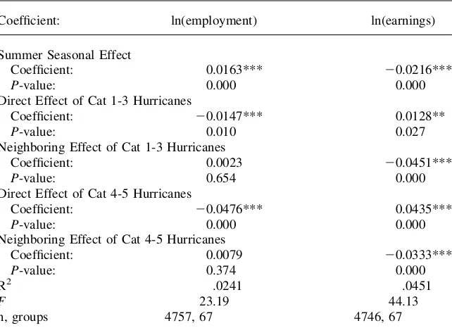
Table 4 outlines the results of these regressions. High-intensity hurricanes have a much greater impact on earnings than we have seen in previous models, as they boost the growth rate of earnings per worker by 4.35 percent on average relative to workers in the average county. There is also a greater magnitude effect on employment, as it drops by 4.76 percent on average relative to the average county. Meanwhile, counties that neighbor the directly hit county will not face an effect on employment from the high-intensity hurricanes, but will experience a 3.33 percent decline in wage growth relative to the typical county. Low-intensity hurricanes, on the other hand, will rel-atively decrease employment by just 1.47 percent and boost earnings growth by 1.28 percent on average in directly hit counties. In neighboring counties, they will de-crease to the average earnings growth rate by 4.51 percent. As such, it appears that more severe storms have a greater impact on the labor market.
B. Timing Effects
Another extension that can be made is to examine the impact of hurricanes over time. Equations 9 and 10 can be augmented using a series of hurricane dummy variables that capture the effects of hurricanes over time to see if there is any lasting impact. The vectorH~D¼ ðHDit;HDit21;HitD22;.Þis used to represent the series of direct effects andH~N¼ ðHN
ijt;HijtN21;HijtN22;.Þto reflect the neighboring effects. Subscripti
indi-cates that the hurricane is directly affecting countyi, the lag indicates how far back in
time the hurricane hit, and subscriptijindicates that a hurricane from countyjaffects
countyi. The coefficients for each of these vectors are vectors themselves, and thus
the model now takes the form:
ðDlnQit2DlnQtÞ ¼a1DSt+DH~itD~ak+DH~Nijt~al
ð15Þ
ðDlnyit2DlnytÞ ¼d1DSt+DH~Dit~dk+DH~ijtN~dl
ð16Þ
As mentioned, according to Lucas and Rapping (1969), one can expect the steady state growth level of earnings to be unaffected by a hurricane event in the long run, but for there to be temporary adjustments in the short run. Guimaraes et al. (1993) found different signs for the initial impact of the hurricanes and for their long-run effects in which Hurricane Hugo impacted South Carolina’s economy. The lagged effects lasted for eight quarters following the hurricane. Furthermore, Ewing et al. (2007) (which only deals with the Oklahoma City tornado) and Ewing and Kruse (2005) (which focuses primarily on Hurricane Bertha) each found that earnings will jump immediately and then converge back toward prehurricane levels; and while hur-ricanes create an economic disturbance in the short run, oftentimes they can lead to economic gains in the long run.
Therefore, the coefficients for the time delayed direct effects should, for the most part, be negative for earnings growth as the values come back down toward their steady state from the hurricane-induced increases, however, we expect the cumulative
effect to yield a slightly positive upswing in earnings to match the findings from earlier papers. Employment, on the other hand, should increase over time as workers return to the rebuilt economy. The neighboring effects occur primarily be-cause labor supply rises as a spillover effect as workers flee hurricane-stricken coun-ties. The influx of workers looking for refuge will lead to a decline in earnings in that county; so one would expect to see earnings rise slightly as some workers relocate
back out of countyi, but the steady state growth level could still wind up lower than
its initial point since many displaced people may never return to their original county.
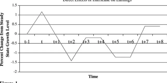
Figures 1 and 2 (below) show the results of the regressions containing the direct
and the neighboring effects of a hurricane in time tas well as the lingering effects
of that hurricane for eight quarters (or 24 months) following the storm.12What the
results imply is that, similar to the time of the hurricane strike, the lagged effects on employment also are likely mitigated by opposing labor market shifts across in-dustries.
Table 4
GDD Regression Results of Hurricanes on Change in the following:
Coefficient: ln(employment) ln(earnings)
Summer Seasonal Effect
Coefficient: 0.0163*** 20.0216***
P-value: 0.000 0.000
Direct Effect of Cat 1-3 Hurricanes
Coefficient: 20.0147*** 0.0128**
P-value: 0.010 0.027
Neighboring Effect of Cat 1-3 Hurricanes
Coefficient: 0.0023 20.0451***
P-value: 0.654 0.000
Direct Effect of Cat 4-5 Hurricanes
Coefficient: 20.0476*** 0.0435***
P-value: 0.000 0.000
Neighboring Effect of Cat 4-5 Hurricanes
Coefficient: 0.0079 20.0333***
P-value: 0.374 0.000
R2 .0241 .0451
F 23.19 44.13
n, groups 4757, 67 4746, 67
Note: Table reports selected coefficients of Equations 13 and 14 fit with QCEW data. See text for details. *Significant at the 10 percent level.
**Significant at the 5 percent level. ***Significant at the 1 percent level.
12. A table of the regression results is available upon request.
The direct effects of an average hurricane are pronounced on earnings growth up through the seventh quarter following the time of the disaster. For neighboring counties, on the other hand, the effects on earnings growth, on average, last into the eighth
quar-ter.13Unlike the Guimaraes et al. (1993) study of Hugo, however, not all of the lags
sig-nificantly impact earnings and employment growth. The disparity can be explained by Ewing and Kruse’s (2006) finding that the effect of a given hurricane is mitigated by the occurrence of other hurricanes within the same time period. If the time delayed effects of one storm coincide with the immediate impact of a second storm, then the effects of both might be difficult to identify and as a result they may be understated in the model. What can be seen in Figure 1 is that a hurricane will immediately boost growth in earnings in the counties where it strikes followed by an immediate downturn one quar-ter laquar-ter. As time goes by, earnings growth will continue to follow this patquar-tern before settling in at a new steady state level roughly 0.40 percent above the level of growth for an average county. While this in no way indicates that earnings growth in a hurricane stricken county will permanently remain higher than in a county that has avoided the hurricane, it does imply that the temporary wage gains may not be as short term as the ones Guimaraes et al. (1993) reported based on Hurricane Hugo. On the other hand, these findings are consistent with the existing literature of Ewing et al. (2007) and Ewing and Kruse (2005) which found that after a hurricane, earnings will jump imme-diately and then converge back toward pre-hurricane levels. Additionally, they find that while hurricanes create an economic disturbance in the short run, oftentimes they can lead to economic gains in the long run, just as we have found in this paper.
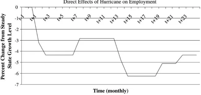
Figure 2 illustrates the cumulative monthly growth rate of employment. We find that the labor market takes a cobweb form in which employment jumps about a year after the hurricane (coinciding with a decrease in earnings) and then decreases as
Figure 1
Average Direct Effects of a Hurricane on Earnings over a Two-Year Duration
13. Ninth and tenth lags were performed as well to verify these findings, and both came up insignificant for each regression.
earnings increase before settling at a growth rate 4.32 percent lower than that of un-affected counties.
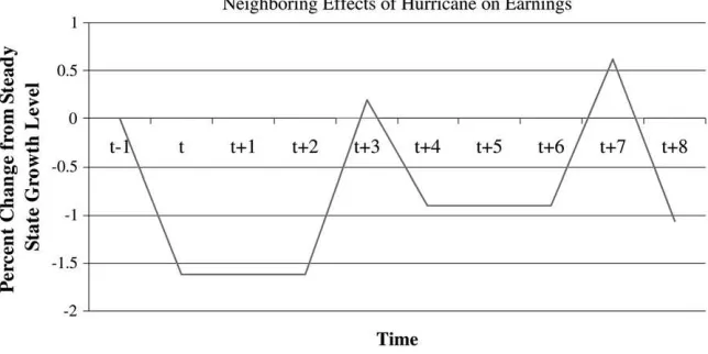
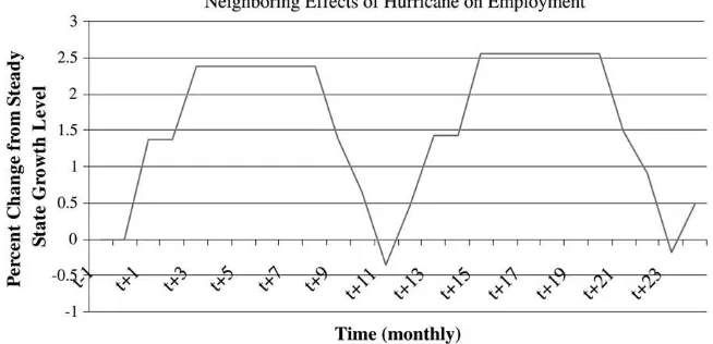
The effects of hurricanes on neighboring counties have similar results, but take a
different course. If a hurricane strikes a county neighboring countyi, earnings growth
will immediately fall in countyiuntil they are roughly 1.62 percent lower on average
than the earnings growth level of a worker in a typical county. It appears as though neighboring counties go through similar earnings changes around the third quarter following the hurricane as do directly hit counties, as wage growth rises above the original level and continues to cycle up and down until two years after the storm to wind up 1.06 percent below the earnings growth level in an average county. Ad-ditionally, as with the directly hit counties, employment in neighboring counties mir-rors earnings in those counties. It too appears to take a cobweb format, where an increase in earnings corresponds with a decrease in employment, and vice versa. Em-ployment growth increases from the initial level; and after cycling along with earn-ings, employment growth ends up 0.49 percent above that of an average unaffected county. (See Figures 3 and 4 below):
At certain points in time, earnings growth will be higher in hurricane-impacted counties than in other counties while employment growth will remain relatively un-changed. This is likely a result of low wage earners being replaced by high-wage earners in the specified counties. Card (1990) and Belasen and Polachek (2008) each
have results that are consistent with these findings.14
Figure 2
Average Direct Effects of a Hurricane on Employment over a Two-Year Duration
14. Other time-related applications that can be drawn from this particular regression are to see if specific time-related events (such as elections or the September 11 terror attack) had any impact on the hurricane effects. As with the additional specifications for intensity effects, these additional time-related effects were also insignificant. However, it appears that timing within a quarter can alter the impact of a hurricane on the labor market, such that hurricanes that occur early on in the quarter will have less of an effect than other hurricanes. This is likely due to the fact that hurricanes last for a week at most and are typically dealt with soon after (see Models 6 and 7 in Tables 2 and 3).
C. Geographic Effects
Thus far, we have studied the effects of hurricanes on three separate groups of counties in Florida: those that were directly hit by the storm, those neighboring the counties that were directly hit, and all other counties. Theoretically speaking we expect that the neighboring effect should diminish with distance, so a town lo-cated 100 miles away from a directly hit county should face a stronger neighbor-ing effect than a town located 200 miles away since the floodneighbor-ing will be greater as the proximity to the locus of destruction increases. To verify this expectation, we fit Equations 9 and 10 with a ‘‘Second County Away’’ variable to capture the effects of hurricanes on the counties located two counties away from the directly hit counties:
ðDlnQit2DlnQtÞ ¼a1DSt+a2DHitD+a3DHNijt+a4DHikt2
ð17Þ
ðDlnyit2DlnytÞ ¼d1DSt+d2DHDit +d3DH N ijt+d4DH
2 ikt
ð18Þ
The new variableDHikt2 takes a value of one for countyiwhen a hurricane strikes
countyk if that countykis two counties away from countyi. In other words, it is
essentially the neighboring effect of the original neighboring effect. One would, therefore, expect to see the coefficients for the neighboring effect and the second-county-away effect to take the same sign, but for the second-second-county-away coefficient to be smaller in magnitude (or insignificant as the case may be). Model 8 in Tables 2 and 3 report the results of these regressions.
Similar to the neighboring effect, the two-away effect is insignificant for employ-ment. In fact, the neighboring effect and the second-county-away effect on average earnings are nearly identical in sign and magnitude. However, the
second-county-Figure 3
Average Neighboring Effects of a Hurricane on Earnings over a Two-Year Duration
away effect is less significant, thus one can argue that it holds up to the theoretical expectations. In addition, we find that the second-county-away effect is insignificant which also verifies expectations. In sum, we are able to conclude from this that the neighboring effect of hurricanes found in earnings diminishes with distance from the path of the storm.
A final extension incorporates geographic location into the model to examine whether certain areas of Florida are affected more heavily by hurricanes than others. To that end, we differentiate between coastal and landlocked counties, as well as between counties located on the Panhandle or in the rest of the state. Coastal counties experience more flooding than landlocked counties and gener-ally find themselves facing higher monetary costs for rebuilding. The hurricane effects, therefore, should be more pronounced for coastal counties. Panhandle counties draw most of their economic growth from tourism whereas other coun-ties tend to have a better developed industrial infrastructure. Therefore we ex-pect to see weaker increases in earnings for directly hit Panhandle counties and stronger decreases for neighboring Panhandle counties since tourism reve-nues are likely to diminish all across the Panhandle after a hurricane strikes
there. Equations 9 and 10 are fit with a variableCto distinguish coastal counties
from non-coastal counties and a variablePto distinguish between those counties
lying on the Panhandle versus all other counties. Furthermore, a great deal of Panhandle counties lie on the coast so there is an interaction between the two sets of geographic comparisons. To that end, we also separate out those counties
that meet both qualifications by adding in a series of interaction terms for bothC
and P:
Figure 4
Average Neighboring Effects of Hurricane on Employment over a Two-Year Duration
ðDlnQit2DlnQtÞ ¼a1DSt+a2DHitD+a3DHijtN
+a4Ci+a5Pi+a6ðCiPiÞ
+a7ðDHitDCiÞ+a8ðDHijtNCiÞ
+a9ðDHitDPiÞ+a10ðDHijtNPiÞ
+a11ðDHitDCiPiÞ+a12ðDHijtNCiPiÞ
ð19Þ
ðDlnyit2DlnytÞ ¼d1DSt+d2DHitD+d3DHijtN
+d4Ci+d5Pi+d6ðCiPiÞ
+d7ðDHDit CiÞ+d8ðDHijtNCiÞ
+d9ðDHDit PiÞ+d10ðDHijtNPiÞ
+d11ðDHitDCiPiÞ+d12ðDHNijtCiPiÞ
ð20Þ
Models 9, 10, and 11 in Tables 2 and 3 each fit the original model with the coastal and/or Panhandle variables (independently as well as together) and their interactions with the hurricanes. Coastal counties and Panhandle counties tend to have a lower change in employment than the rest of the state. However, the impact of hurricanes on employment does not appear to be any different across the different geographic classifications. Both coastal and Panhandle counties also exhibit a greater increase in earnings than the rest of the state. And while there is no discernable difference between the different types of counties after a direct hit from a hurricane, neighbor-ing effects change drastically by isolatneighbor-ing the geographic characteristics of the county.
Explicitly accounting for the Panhandle in Models 10 and 11 appears to somewhat negate the overall effects of hurricanes on the average neighboring county. Whereas
theDHijtN coefficient becomes insignificant, the interaction term between the
Panhan-dle and the neighboring hurricane variables is significantly negative. This implies that neighbors of Panhandle counties are the counties most affected by hurricanes. Relative earnings in these counties fall 3.21 to 5.31 percent when their neighbors in the Panhandle are hit by a hurricane. Neighbors of coastal states hit by a hurricane are negligibly affected as earnings fall only by -0.01 percent (Models 9 and 11). Fi-nally, the magnitude of employment effects is much greater for both direct and neighboring counties relative to the typical county if those hurricane-impacted coun-ties lie both along the coast and the Panhandle.
VI. Conclusion
As illustrated by hurricanes, exogenous shocks to an economy will lead to opposing shifts in wages and the size of the labor force across neighboring local labor markets. Therefore, exogenous factors that may not appear to have much of an impact on a macro scale, may yet play a major role in shaping the differences across local markets.
The devastation and frequency of hurricanes in the North Atlantic Ocean is unpar-alleled relative to other natural disasters in the United States. The widespread devas-tation of hurricanes can wipe out infrastructure, private homes, businesses, and even entire communities. While the effects can be measured by looking directly at the loss of life and damage to property, there are also indirect results of a hurricane. One such result is the effect of hurricanes on local labor markets. This paper developed a GDD model that, through various specifications, isolated two distinct effects hurricanes have on labor markets. The first involves the specific counties directly struck by hur-ricanes. Here the hurricane decreases employment in the stricken counties while at the same time boosting earnings, thus appearing to negatively impact labor supply, while at the same time changing the labor demand for certain industrial sectors. And as workers flee the devastation by heading into neighboring counties, those counties experience a positive labor supply shock moving the equilibrium downward along what appears to be a perfectly inelastic labor demand curve. The result is that employment is relatively unchanged, while earnings will have declined.
We find that as a portion of the labor force flees a hurricane-stricken county, the growth of earnings per worker remaining in that county of Florida will increase up to 4.35 percent relative to workers outside that county. Meanwhile, as workers flow into nearby counties, the growth of earnings per worker in those regions will decrease by as much as 4.51 percent. Even two years after the hurricane, earnings may still re-main higher in areas hit by a hurricane than elsewhere.
Particularly in today’s age of increased intensity, duration, and sheer quantity of tropical storms, policymakers looking to rebuild hurricane damaged economies can point to the wage benefits for workers who relocate to regions that have been hit by hurricanes. This entails both short-term and long-term effects on both direct-ly hit and neighboring counties, which we find to exhibit somewhat of a cobweb quarter-by-quarter. These findings should help policy makers assess such issues as UI eligibility. In addition, it should help policy makers in areas outside of the South-east US such as California, Mexico, and Brazil that are now being hit by hurricanes due to recent weather changes.
Subsequent studies related to Generalized Difference-in-Difference could include the examination of the impact of unplanned illegal immigration on local economies or the influx of a new disease. In addition, the exogenous effects of other natural di-sasters (for example earthquakes, tornados, tsunamis, etc.) could also be captured by this model using the same framework. Finally, other variables of study could include FEMA funding and other economic specifications (such as GDP growth, consumer spending, industrial growth, etc.).
References
Abadie, Alberto, Alexis Diamond, and Jens Hainmueller. 2007. ‘‘Synthetic Control Methods for Comparative Case Studies: Estimating the Effect of California’s Tobacco Control Problem.’’ NBER Working Paper 12831.
Angrist, Joshua A., and Alan B. Krueger. 1999. ‘‘Empirical Strategies in Labor Economics.’’ InHandbook of Labor Economics3A, ed. Orley C. Ashenfelter and David A. Card, 1277-1366. Amsterdam: Elsevier.
Avila, Lixion A. 1999. ‘‘Preliminary Report: Hurricane Irene.’’National Oceanic and Atmospheric Association.http://www.nhc.noaa.gov/1999irene.html.
Belasen, Ariel R., and Solomon W. Polachek. 2007. ‘‘How Hurricanes Affect Wages and Employment in Local Labor Markets.’’American Economic Review98(2):49-53. Bertrand, Marianne, Esther Duflo, and Sendhil Mullainathan. 2002. ‘‘How Much Should We
Trust Differences-in-Differences Estimates?’’ NBER working paper 8841.
Beven, John L. II. 2004. ‘‘Tropical Cyclone Report: Hurricane Frances,’’National Oceanic and Atmospheric Association.http://www.nhc.noaa.gov/2004frances.shtml.
__________. 2006. ‘‘Tropical Cyclone Report: Hurricane Dennis.’’National Oceanic and Atmospheric Association, http://www.nhc.noaa.gov/pdf/TCR-AL042005_Dennis.pdf. Beven, John L., II., and Hugh D. Cobb. 2006. ‘‘Tropical Cyclone Report: Hurricane Ophelia.’’
National Oceanic and Atmospheric Association, http://www.nhc.noaa.gov/pdf/TCR-AL162005_Ophelia.pdf.
Card, David. 1990. ‘‘The Impact of the Marial Boatlift on the Miami Labor Market.’’
Industrial and Labor Relations Review43(2):245-257.
Climate.org. 2004. ‘‘Brazil Hurricane.’’ http://www.climate.org/topics/climate/ brazil_hurricane.shtml.
Connolly, Marie. 2007. ‘‘Here Comes the Rain Again: Weather and Intertemporal Substitution of Leisure.’’ Princeton: Princeton University.
Ewing, Bradley T., and Jamie B. Kruse. 2005. ‘‘Hurricanes and Unemployment.’’ Center for Natural Hazards Research. Greenville: East Carolina University.
Ewing, Bradley T., Jamie B. Kruse, and Mark A. Thompson. 2007. ‘‘Twister! Employment Responses to the May 3, 1999, Oklahoma City Tornado.’’Journal of Applied Economics
Forthcoming.
Google. 2006. ‘‘Google Earth.’’ http://earth.google.com.
Guimaraes, Paulo, Frank L. Hefner, and Douglas P. Woodward. 1993. ‘‘Wealth and Income Effects of Natural Disasters: An Econometric Analysis of Hurricane Hugo.’’The Review of Regional Studies23:97-114.
Guiney, John L. 1999. ‘‘Preliminary Report: Hurricane Georges.’’National Oceanic and Atmospheric Association, http://www.nhc.noaa.gov/1998georges.html.
Knabb, Richard D., Jaime R. Rhome, and Daniel P. Brown. 2005. ‘‘Tropical Cyclone Report: Hurricane Katrina.’’National Oceanic and Atmospheric Association, http://
www.nhc.noaa.gov/pdf/TCR-AL122005_Katrina.pdf.
__________. 2006. ‘‘Tropical Cyclone Report: Hurricane Rita.’’National Oceanic and Atmospheric Association, http://www.nhc.noaa.gov/pdf/TCR-AL182005_Rita.pdf. Kubik, Jeffrey D., and John Moran. 2003. ‘‘Can Policy Changes be Treated as Natural
Experiments?’’ Evidence from Cigarette Excise Taxes." SSRN working paper 269609. Lawrence, Miles B., and Hugh D. Cobb. 2005. ‘‘Tropical Cyclone Report: Hurricane Jeanne.’’
National Oceanic and Atmospheric Association, http://www.nhc.noaa.gov/2004jeanne. shtml.
Lucas, Robert E., and Leonard A. Rapping. 1969. ‘‘Price Expectations and the Phillips Curve.’’The American Economic Review59(3):342-50.
Mayfield, Max. 1995. ‘‘Preliminary Report: Hurricane Opal.’’National Oceanic and Atmospheric Association, http://www.nhc.noaa.gov/1995opal.html.
__________. 1998. ‘‘Preliminary Report: Hurricane Earl.’’National Oceanic and Atmospheric Association, http://www.nhc.noaa.gov/1998earl.html.
Miguel, Edward. 2005. ‘‘Poverty and Witch Killing.’’Review of Economic Studies
72(4):1153-72.
National Oceanic and Atmospheric Association. 1988. ‘‘Hurricane Florence.’’ http:// www.hpc.ncep.noaa.gov/tropical/rain/florence1988.html.
__________. 2006. ‘‘Hurricanes.’’ http://hurricanes.noaa.gov/.
__________. 2006. ‘‘Retired Hurricane Names.’’ http://www.nhc.noaa.gov/ retirednames.shtml.
Padgett, Gary, Jack Beven, and James L. Free. 2004. ‘‘FAQ: Hurricanes, Typhoons, and Tropical Cyclones.’’Atlantic Oceanographic and Meteorological Laboratory, National Oceanic and Atmospheric Association, http://www.aoml.noaa.gov/hrd/tcfaq/B3.html. Pasch, Richard J. 1996. ‘‘Preliminary Report: Hurricane Allison.’’National Oceanic and
Atmospheric Association, http://www.nhc.noaa.gov/1995allison.html.
__________. 1997. ‘‘Preliminary Report: Hurricane Danny.’’National Oceanic and Atmospheric Association, http://www.nhc.noaa.gov/1997danny.html.
Pasch, Richard J., Eric S. Blake, Hugh D. Cobb, and David P. Roberts. 2006. ‘‘Tropical Cyclone Report: Hurricane Wilma.’’National Oceanic and Atmospheric Association, http://www.nhc.noaa.gov/pdf/TCR-AL252005_Wilma.pdf.
Pasch, Richard J., Daniel P. Brown, and Eric S. Blake. 2005. ‘‘Tropical Cyclone Report: Hurricane Charley.’’National Oceanic and Atmospheric Association, http://
www.nhc.noaa.gov/2004charley.shtml.
Pew Center on Global Climate Change. 2006. ‘‘Global Warming and Hurricanes,’’ http:// www.pewclimate.org/hurricanes.cfm/.
Rappaport, Ed. 1993. ‘‘Preliminary Report: Hurricane Andrew.’’National Oceanic and Atmospheric Association, http://www.nhc.noaa.gov/1992andrew.html.
__________. 1995. ‘‘Preliminary Report: Hurricane Erin.’’National Oceanic and Atmospheric Association, http://www.nhc.noaa.gov/1995erin.html.
Skidmore, Mark, and Hideki Toya. 2002. ‘‘Do Natural Disasters Promote Long-Run Growth?’’Economic Inquiry40:664–687.
Stewart, Stacy R. 2001. ‘‘Preliminary Report: Hurricane Gordon.’’National Oceanic and Atmospheric Association, http://www.nhc.noaa.gov/2000gordon.html.
__________. 2005. ‘‘Tropical Cyclone Report: Hurricane Ivan.’’National Oceanic and Atmospheric Association, http://www.nhc.noaa.gov/2004ivan.shtml.
U.S. Geological Survey. 2006. ‘‘SOFIA: South Florida Information Access.’’ http:// sofia.usgs.gov.
Waldman, Michael, Sean Nicholson, and Nodir Adilov. 2006. ‘‘Does Television Cause Autism?’’ NBER working paper 12632.