Full Terms & Conditions of access and use can be found at
http://www.tandfonline.com/action/journalInformation?journalCode=ubes20
Download by: [Universitas Maritim Raja Ali Haji] Date: 12 January 2016, At: 00:21
Journal of Business & Economic Statistics
ISSN: 0735-0015 (Print) 1537-2707 (Online) Journal homepage: http://www.tandfonline.com/loi/ubes20
Modeling Financial Return Dynamics via
Decomposition
Stanislav Anatolyev & Nikolay Gospodinov
To cite this article: Stanislav Anatolyev & Nikolay Gospodinov (2010) Modeling Financial Return Dynamics via Decomposition, Journal of Business & Economic Statistics, 28:2, 232-245, DOI: 10.1198/jbes.2010.07017
To link to this article: http://dx.doi.org/10.1198/jbes.2010.07017
Published online: 01 Jan 2012.
Submit your article to this journal
Article views: 218
Modeling Financial Return Dynamics
via Decomposition
Stanislav ANATOLYEV
New Economic School, Nakhimovsky Pr. 47, Moscow 117418, Russia (sanatoly@nes.ru)
Nikolay GOSPODINOV
Department of Economics, Concordia University, 1455 de Maisonneuve Blvd. West, Montreal, Quebec H3G 1M8, Canada (gospodin@alcor.concordia.ca)
While the predictability of excess stock returns is detected by traditional predictive regressions as sta-tistically small, the direction-of-change and volatility of returns exhibit a substantially larger degree of dependence over time. We capitalize on this observation and decompose the returns into a product of sign and absolute value components whose joint distribution is obtained by combining a multiplicative error model for absolute values, a dynamic binary choice model for signs, and a copula for their interaction. Our decomposition model is able to incorporate important nonlinearities in excess return dynamics that cannot be captured in the standard predictive regression setup. The empirical analysis of U.S. stock return data shows statistically and economically significant forecasting gains of the decomposition model over the conventional predictive regression.
KEY WORDS: Absolute returns; Copulas; Directional forecasting; Joint predictive distribution; Stock returns predictability.
1. INTRODUCTION
It is now widely believed that excess stock returns exhibit a certain degree of predictability over time (Cochrane2005). For instance, valuation (dividend-price and earnings-price) ratios (Campbell and Shiller1988; Fama and French1988) and yields on short and long-term U.S. Treasury and corporate bonds (Campbell 1987) appear to possess some predictive power at short horizons that can be exploited for timing the market and active asset allocation (Campbell and Thompson 2008; Tim-mermann 2008). Given the great practical importance of pre-dictability of excess stock returns, there is a growing recent lit-erature in search of new variables with incremental predictive power, such as share of equity issues in total new equity and debt issues (Baker and Wurgler2000), consumption-wealth ra-tio (Lettau and Ludvigson2001), relative valuations of high and low-beta stocks (Polk, Thompson, and Vuolteenaho2006), esti-mated factors from large economic datasets (Ludvigson and Ng
2007), etc. Lettau and Ludvigson (2008) provide a comprehen-sive review of this literature. In this paper, we take an alternative approach to predicting excess returns: instead of trying to iden-tify better predictors, we look for better ways of using predic-tors. We accomplish this by modeling individual multiplicative components of excess stock returns and combining information in the components to recover the conditional expectation of the original variable of interest.
To fix ideas, suppose that we are interested in predicting ex-cess stock returns on the basis of past data and letrtdenote the excess return at periodt. The return can be factored as
rt= |rt|sign(rt),
which is called “an intriguing decomposition” in Christoffersen and Diebold (2006). The conditional mean ofrt is then given by
Et−1(rt)=Et−1(|rt|sign(rt)),
whereEt−1(·)denotes the expectation taken with respect to the available informationIt−1up to timet−1. Our aim is to model the joint distribution of absolute values|rt|and signs sign(rt)in order to pin down the conditional expectationEt−1(rt). The ap-proach we adopt to achieve this involves joint usage of a mul-tiplicative error model for absolute values, a dynamic binary choice model for signs, and a copula for their interaction. We expect this detour to be successful for the following reasons.
First, the joint modeling of the multiplicative components is able to incorporate important hidden nonlinearities in excess return dynamics that cannot be captured in the standard pre-dictive regression setup. In fact, we argue that a conventional predictive regression lacks predictive power when the data are generated by ourdecomposition model. Second, the absolute values and signs exhibit a substantial degree of dependence over time while the predictability of returns seems to be statis-tically small as detected by conventional tools. Indeed, volatil-ity (as measured by absolute values of returns) persistence and predictability has been extensively studied and documented in the literature (for a comprehensive review, see Andersen et al.
2006). More recently, Christoffersen and Diebold (2006), Hong and Chung (2003), and Linton and Whang (2007) find con-vincing evidence of sign predictability of U.S. stock returns for different data frequencies. Of course, the presence of sign and volatility predictability is not sufficient for mean predictability: Christoffersen and Diebold (2006) show that sign predictability may exist in the absence of mean predictability, which helps to reconcile the standard finding of weak conditional mean pre-dictability with possibly strong sign and volatility dependence. Note that the joint predictive distribution of absolute values and signs provides a more general inference procedure than
© 2010American Statistical Association
Journal of Business & Economic Statistics April 2010, Vol. 28, No. 2 DOI:10.1198/jbes.2010.07017
232
modeling directly the conditional expectation of returns as in the predictive regression literature. Studying the dependence between the sign and absolute value components over time is interesting in its own right and can be used for various other purposes. One important aspect of the bivariate analysis is that, in spite of a large unconditional correlation between the mul-tiplicative components, they appear to be conditionally very weakly dependent.
As a by-product, the joint modeling would allow the re-searcher to explore trading strategies and evaluate their prof-itability (Satchell and Timmermann1996; Qi1999; Anatolyev and Gerko2005), although an investment strategy requires in-formation only about the predicted direction of returns. In our empirical analysis of U.S. stock return data we perform a sim-ilar portfolio allocation exercise. For example, with an initial investment in 1952 of $100 that is reinvested every month ac-cording to predictions of the models, the value of the portfo-lios in 2002, after accounting for transaction costs, is $80,430 for the decomposition model, $62,516 for the predictive regres-sion, and $20,747 for the buy-and-hold strategy. Interestingly, the decomposition model succeeds out-of-sample in the 1990s for which period the forecast breakdown of the standard predic-tive regression is well documented. Finally, the decomposition model produces unbiased forecasts of next period excess re-turns while the forecasts based on the predictive regression and historical average appear to be biased.
The rest of the paper is organized as follows. In Section2, we introduce our return decomposition, discuss the marginal density specifications and construction of the joint predictive density of sign and absolute value components, and demon-strate how mean predictions can be generated. Section3 con-tains an empirical analysis of predictability of U.S. excess re-turns. In this section, we present the results from the decom-position model, provide in-sample and out-of-sample statistical comparisons with the benchmark predictive regression, eval-uate the performance of the models in the context of a port-folio allocation exercise, and report some simulation evidence about the inability of the linear regression to detect predictabil-ity when the data are generated by the decomposition model. In Section4, we present our conclusion.
2. METHODOLOGICAL FRAMEWORK
2.1 Decomposition and Its Motivation
The key identity that lies in the heart of our technique is the return decomposition
rt=c+ |rt−c|sign(rt−c)
=c+ |rt−c|(2I[rt>c] −1), (1) whereI[·]is the indicator function andcis a user-determined constant. Ourdecomposition modelwill be based on the joint dynamic modeling of the two ingredients entering (1), the ab-solute values|rt−c|andindicatorsI[rt>c](or, equivalently, signssign(rt−c)related linearly to indicators). In case the in-terest lies in the mean prediction of returns, one can infer from (1) that
Et−1(rt)=c−Et−1(|rt−c|)+2Et−1(|rt−c|I[rt>c]),
and the decomposition model can be used to generate optimal predictions of returns because it allows to deduce, among other things, the conditional mean of|rt−c|and conditional expected cross-product of |rt −c| and I[rt>c] (for details, see Sec-tion2.4). In a different context, Rydberg and Shephard (2003) use a decomposition similar to (1) for modeling the dynamics of the trade-by-trade price movements. The potential usefulness of decomposition (1) is also stressed in Granger (1998) and Ana-tolyev and Gerko (2005).
Recall that c is a user-determined constant. Although our empirical analysis only considers the leading case c=0, we develop the theory for arbitrary c for greater generality. The choice ofcis dictated primarily by the application at hand. In the context of financial returns, Christoffersen and Diebold (2006) analyze the case when c=0 while Hong and Chung (2003) and Linton and Whang (2007) use threshold values forc
that are multiples of the standard deviation ofrtor quantiles of the marginal distribution ofrt. The nonzero thresholds may re-flect the presence of transaction costs and capture possible dif-ferent dynamics of small, large positive, and large negative re-turns (Chung and Hong2007). In macroeconomic applications, in particular modeling GDP growth rates,cmay be set to 0 if one is interested in recession/expansion analysis, or to 3%, for instance, if one is interested in modeling and forecasting a po-tential output gap. Likewise, it seems natural to setcto 2% if one considers modeling and forecasting inflation.
To provide further intuition and demonstrate the advantages of the decomposition model, consider a toy example in which we try to predict excess returns rt with the lagged realized volatilityRVt−1. A linear predictive regression ofrtonRVt−1, estimated on data from our empirical section, gives in-sample
R2=0.39%. Now suppose that we employ a simple version of the decomposition model where the same predictor is used lin-early for absolute values, that is,Et−1(|rt|)=α|r|+β|r|RVt−1, and for indicators in a linear probability model Prt−1(rt>0)= αI+βIRVt−1. Assume for simplicity that the shocks in the two components are stochastically independent. Then, it is easy to see from identity (1) thatEt−1(rt)=αr+βrRVt−1+γrRV2t−1 for certain constantsαr, βr, andγr. Running a linear predic-tive regression on both RVt−1 andRV2t−1 yields a much bet-ter fit withR2=0.72% (even a linear predictive regression on
RV2t
−1alone givesR2=0.69%, which indicates thatRV2t−1is a much better predictor thanRVt−1). Further, addingI[rt−1>0] andRVt−1I[rt−1>0]to the regressor list, which is implied by augmenting the model for indicators or the model for absolute values byI[rt−1>0], drivesR2up to 1.21%! These examples clearly suggest that the conventional predictive regression may miss important nonlinearities that are easily captured by the de-composition model.
Alternatively, suppose that the true model for indicators is trivial, that is, Prt−1(rt>0)=αI=12, and the components are conditionally independent. Then, using again identity (1), it is straightforward to see that any parameterization of expected ab-solute valuesEt−1(|rt|)leads to the same form of parameteriza-tion of the predictive regressionEt−1(rt). Augmenting the para-meterization for indicators and accounting for the dependence between the multiplicative components then automatically de-livers an improvement in the prediction ofrtby capturing hid-den nonlinearities in its dynamics.
While the model setup used in the above example is fairly simplified (indeed, the regressors RV2t, I[rt−1 > 0] and RVt−1I[rt−1>0] are quite easy to find), the arguments that favor the decomposition model naturally extend to more com-plex settings. In particular, when the component models are quite involved and the components themselves are condition-ally dependent, we find via simulations that the standard linear regression framework has difficulties detecting any perceivable predictability as judged by the conventional criteria (see Sec-tion3.6). The driving force behind the predictive ability of the decomposition model is the predictability in the two compo-nents, documented in previous studies. Note also that, unlike the example above, the models for absolute values and indica-tors may in fact use different information variables.
2.2 Marginal Distributions
Consider first the model specification for absolute returns. Since |rt−c| is a positively valued variable, the dynamics of absolute returns is specified using the multiplicative error mod-eling (MEM) framework of Engle (2002):
|rt−c| =ψtηt,
where ψt =Et−1(|rt−c|) andηt is a positive multiplicative error withEt−1(ηt)=1 and conditional distributionD. Engle (2002), Chou (2005), and Engle and Gallo (2006) use the MEM methodology for volatility modeling, while Anatolyev (2009) applies it in the context of asymmetric loss; however, the main application of the MEM approach is the analysis of durations between successive transactions in financial markets (Engle and Russel1998).
The conditional expectationψt and conditional distribution
D of |rt −c| can be parameterized following the sugges-tions in the MEM literature (Engle and Russell 1998; Engle
2002). A convenient dynamic specification for ψt is the log-arithmic autoregressive conditional duration (LACD) model of Bauwens and Giot (2000) whose main advantage, espe-cially when (weakly) exogenous predictors are present, is that no parameter restrictions are needed to enforce positivity of
Et−1(|rt−c|). Possible candidates forD include exponential, Weibull, Burr, and Generalized Gamma distributions, and po-tentially the shape parameters ofD may be parameterized as
functions of the past. In the empirical section, we use the con-stant parameter Weibull distribution as it turns out that its flexi-bility is sufficient to provide an adequate description of the con-ditional density of absolute excess returns. Let us denote the vector of shape parameters ofDbyς.
The conditional expectationψtis parameterized as
lnψt=ωv+βvlnψt−1+γvln|rt−1−c|
+ρvI[rt−1>c] +x′t−1δv. (2) If only the first three terms on the right-hand side of (2) are in-cluded, the structure of the model is analogous to the LACD model of Bauwens and Giot (2000) and the log GARCH model of Geweke (1986) where the persistence of the process is mea-sured by the parameter |γv+βv|. We also allow for regime-specific mean volatility depending on whether rt−1 >c or rt−1≤c. Finally, the termx′t−1δv accounts for the possibility
that macroeconomic predictors such as valuation ratios and in-terest rates variables may have an effect on volatility dynamics proxied by|rt−c|. In what follows, we refer to model (2) as thevolatility model.
Now we turn our attention to the dynamic specification of the indicator I[rt >c]. The conditional distribution of
I[rt>c], given past information, is of course BernoulliB(pt) difference with unit variance and distribution function Fε(·), Christoffersen and Diebold (2006) show that
Prt−1(rt>c)=1−Fε
This expression suggests that time-varying volatility can gen-erate sign predictability as long as c−μt =0. Furthermore, Christoffersen et al. (2007) derive a Gram–Charlier expansion of Fε(·)and show that Prt−1(rt>c)depend on the third and fourth conditional cumulants of the standardized errorsεt. As a result, sign predictability would arise from time variability in second and higher-order moments. We use these insights and parameterizeptas a dynamic logit model
pt=
exp(θt) 1+exp(θt) with
θt=ωd+φdI[rt−1>c] +y′t−1δd, (3) where the set of predictorsyt−1includes macroeconomic vari-ables (valuation ratios and interest rates) as well as realized measures such as realized variance (RV), bipower variation (BPV), realized third (RS) and fourth (RK) moments of re-turns as suggested above. We experimented with some flexi-ble nonlinear specifications ofθt in order to capture the pos-sible interaction between volatility and higher-order moments (Christoffersen et al.2007) but the nonlinear terms did not de-liver incremental predictive power and are omitted from the fi-nal specification. We include bothRV andBPV as proxies for the unobserved volatility process since the former is an estima-tor of integrated variance plus a jump component while the lat-ter is unaffected by the presence of jumps (Barndorff-Nielsen and Shephard 2004). The conditions for consistency and as-ymptotic normality of the parameter estimates in the dynamic binary choice model (3) are provided in de Jong and Woutersen (2005). In what follows, we refer to model (3) as thedirection model.
Of course, in other applications of the decomposition method, different specifications forψt,D, andptare possibly necessary, depending on the empirical context.
2.3 Joint Distribution Using Copulas
This subsection discusses the construction of the bivariate conditional distribution ofRt≡(|rt−c|,I[rt>c])′ whose do-main isR+× {0,1}. Up to now we have dealt with the
(condi-tional) marginals of the two components:
with marginal PDF/PMFs
If the two marginals were normal, a reasonable thing to do would be to postulate bivariate normality. If the two were ex-ponential, a reasonable parameterization would be joint expo-nentiality. Unfortunately, even though the literature documents a number of bivariate distributions with marginals from differ-ent families (e.g., Marshall and Olkin1985), it does not sug-gest a bivariate distribution whose marginals are Bernoulli and, say, exponential. Therefore, to generate the joint distribution from the specified marginals we use the copula theory (for in-troduction to copulas, see Nelson1999and Trivedi and Zimmer
2005, among others). Denote byFRt(u,v)andfRt(u,v)the joint CDF/CMF and joint density/mass ofRt, respectively. Then, in particular, The unusual feature of our setup is the continuity of one mar-ginal and the discreteness of the other, while the typical case in bivariate copula modeling are two continuous marginals (e.g., Patton 2006) and, much more rarely, two discrete marginals (e.g., Cameron et al.2004). For our case, we derive the fol-lowing result.
Theorem. The joint density/mass function fRt(u,v) can be represented as
Proof. Because the first component is continuously distrib-uted while the second component is a zero-one random vari-able, the joint density/mass function is
fRt(u,v)=
Differentiation ofFRt(u,v)yields
fRt(u,v)=f|rt−c|(u)
while when evaluated atv=1 it is equal to
1−∂C(F
D(u|ψ
t),1−pt)
∂w1 .
Now the conclusion easily follows.
The representation (4) for the joint density/mass function has the form of a product of the marginal density of|rt−c| and the “deformed” Bernoulli mass of I[rt >c]. The “deformed” Bernoulli success probability ̺t(FD(u|ψt)) does not, in gen-eral, equal to the marginal success probabilitypt(equality holds in the case of conditional independence between|rt−c| and
I[rt>c]); it depends not only on pt, but also on FD(u|ψt), which induces dependence between the marginals. Interest-ingly, the form of representation (4) does not depend on the marginal distribution of|rt−c|, although the joint density/mass function itself does.
Below we list three choices of copulas that will be used in the empirical section. The literature contains other examples (Trivedi and Zimmer 2005). Let us denote the vector of cop-ula parameters byα; usuallyαis one-dimensional and indexes dependence between the two marginals.
Frank copula. The Frank copula is
C(w1,w2)= − (positive) dependence. The joint density/mass function is given in (4) with
Note thatα→0 implies independence between the marginals and̺t→pt.
Clayton copula. The Clayton copula is
C(w1,w2)=(w−1α+w−2α−1)−1/α, note that this copula permits only positive dependence between the marginals, which should not be restrictive for our applica-tion.
Farlie–Gumbel–Morgenstern copula. The Farlie–Gumbel– Morgenstern (FGM) copula is
C(w1,w2)=w1w2(1+α(1−w1)(1−w2)),
whereα∈ [−1,+1]andα <0 (α >0) implies negative (pos-itive) dependence. Note that this copula is useful only when the dependence between the marginals is modest, which again turns out not to be restrictive for our application. The joint den-sity/mass is as (4) with
̺t(z)=1−(1−pt)(1+αpt(1−2z)).
Finally,α=0 implies independence between the marginals and
̺t=pt.
Once all the three ingredients of the joint distribution ofRt, that is, the volatility model, the direction model, and the copula, are specified, the vector (ωv, βv, γv, ρv, δv′, ς′, ωd, φd, δ′d, α′)′ can be estimated by maximum likelihood. From (4), the sam-ple log-likelihood function to be maximized is given by
T
In many cases, the interest lies in the mean prediction of re-turns that can be expressed as
Et−1(rt)=c+Et−1
|rt−c|(2I[rt>c] −1)
=c−Et−1(|rt−c|)+2Et−1(|rt−c|I[rt>c]). Hence, the prediction of returns at timetis given by
rt=c−ψt+2ξt, (5)
and the returns can be predicted by
rt=c+(2pt−1)ψt, (6) wherept denotes the feasible value of pt. Note that one may ignore the dependence and use forecasts constructed as (6) even under conditional dependence between the components, but such forecasts will not be optimal. However, as it happens in our empirical illustration, if this conditional dependence is weak, the feasible forecasts (6) may well dominate the feasible optimal forecasts (5).
In the rest of this subsection, we discuss a technical sub-tlety of computing the conditional expected cross-productξt= Et−1(|rt−c|I[rt>c])in the general case of conditional
depen-Then, the conditional expectation function of I[rt >c] given
|rt−c|is
and the expectation of the cross-product is given by
ξt=Et−1(|rt−c|I[rt>c])
=
+∞
0
ufD(u|ψt)̺t(FD(u|ψt))du. (7)
In general, the integral (7) cannot be computed analytically (even in the simple case when fD(u|ψt)is exponential), but can be evaluated numerically, keeping in mind that the do-main of integration is infinite. Note that the change of variables
z=FD(u|ψt)yields
ξt=
1
0
QD(z)̺t(z)dz, (8)
whereQD(z)is a quantile function of the distributionD. Hence,
the returns can be predicted by (5), whereξt is obtained by numerically evaluating integral (8) with a fitted quantile func-tion and fitted funcfunc-tion̺t(z). In the empirical section, we ap-ply the Gauss–Chebyshev quadrature formulas (Judd1998, sec-tion 7.2) to evaluate (8).
3. EMPIRICAL ANALYSIS
In this section we present an empirical analysis of pre-dictability of U.S. excess returns based on monthly data. We have also studied analogous models for quarterly data and ob-tained similar results. An Appendix containing these results ac-companied by some discussion is available from the website
http:// www.nes.ru/ ~sanatoly/ Papers/ DecompApp.pdf or upon request.
3.1 Data
In our empirical study, we use Campbell and Yogo’s (2006) dataset that covers the period from January 1952 to Decem-ber 2002 at the monthly frequency. The excess stock re-turns and dividend-price ratio (dp) are constructed from the NYSE/AMEX value-weighted index and one-month T-bill rate from the Center for Research in Security Prices (CRSP) data-base. The earnings-price ratio (ep) is computed from S&P500 data and Moody’s Aaa corporate bond yield data are used to obtain the yield spread (irs). We also use the three-month T-bill rate (ir3) from CRSP as a predictor variable. The dividend-price and earnings-price ratios are in logs.
The realized measures of second and higher-order mo-ments of stock returns are constructed from daily data on the NYSE/AMEX value-weighted index from CRSP. Letmbe the number of daily observations per month andrt,jdenote the de-meaned daily log stock return for dayjin periodt. Then, the realized varianceRVt (Andersen and Bollerslev1998; Ander-sen et al.2006), bipower variationBPVt(Barndorff-Nielsen and Shephard2004), realized third momentRStand realized fourth moment RKt for period t are computed as RVt =ms=1r2t,s, BPVt=π2mm−1ms=−11|rt,s||rt,s+1|,RSt=ms=1r3t,s andRKt=
m s=1r4t,s.
3.2 Predictive Regressions for Excess Returns
In this section, we present some empirical evidence on condi-tional mean predictability of excess stock returns from a linear predictive regression model estimated by OLS. In addition to the macroeconomic predictors that are commonly used in the literature, we follow Guo (2006) and include a proxy for stock market volatility (RV) as a predictor of future returns. We also attempted to match exactly the information variables that we use later in the decomposition model but the inclusion of the other realized measures generated large outliers in the predicted returns that deteriorated significantly the predictive ability of the linear model.
It is now well known that if the predictor variables are highly persistent, which is the case with the four macroeconomic pre-dictorsdp,ep,ir3, andirs, the coefficients in the predictive re-gression are biased (Stambaugh1999) and their limiting distri-bution is nonstandard (Elliott and Stock1994) when the inno-vations of the predictor variable are correlated with returns. For example, Campbell and Yogo (2006) report that these correla-tions are−0.967 and−0.982 for dividend-price and earnings-price ratios while the innovations of the three-month T-bill rate and the long-short interest rate spread are only weakly correlated with returns (the correlation coefficients of−0.07). A number of recent papers propose inference procedures that take these data characteristics into account when evaluating the predictive power of the different regressors (Torous and Valka-nov2000; Torous, Valkanov, and Yan2004; Campbell and Yogo
2006; among others).
The first panel of Table 1 reports some regression statis-tics when all the predictors are included in the regression. As argued above, the distribution theory for the t-statistics of the dividend-price and earnings-price ratios is nonstandard whereas thet-statistics for the interest rates variables and real-ized volatility can be roughly compared to the standard normal critical values due to their near-zero correlation with the returns innovations and low persistence, respectively. The results in the last two columns suggest some in-sample predictability with a value of theLRtest statistic for joint significance of 27.8 and anR2of 4.45%. Even though the value of theR2coefficient is small in magnitude, Campbell and Thompson (2008) argue that it can still generate large utility gains for investors. Also, while some of the predictors (realized volatility, 3-month rate, and earning-price ratio) do not appear statistically significant, they help to improve the out-of-sample predictability of the model as will be seen in the out-of-sample forecasting and the portfolio management exercises presented below.
It would be interesting to see if it is possible to accommo-date some of the nonlinearities present in the data by simpler
representations than the decomposition model (recall the dis-cussion in Section2.1). Therefore, we include interaction terms
I[rt−1>0]andRVt−1I[rt−1>0]that arise from interacting the linear specifications of the two components and are expected to increase the predictive power of the model. The results are reported in the second row of Table1. Although the predictive gains appear fairly modest, there is clearly space for enhancing predictive ability by using nonlinear modeling. Another inter-esting observation is that the predictive power ofRVincreases and the impact ofRV on returns seems to differ depending on whether the past returns are positive or negative.
3.3 Decomposition Model for Excess Returns
Before we present the results from the decomposition model, we provide some details regarding the selected specification and estimation procedure. We postulateDto be scaled Weibull
with shape parameterς >0 (the exponential distribution corre-sponds to the special caseς=1),
FD(u|ψt)=1−exp
−(ψt−1Ŵ(1+ς−1)u)ς,
fD(u|ψt)=ψt−ςς Ŵ(1+ς−1)ςuς−1
×exp−(ψt−1Ŵ(1+ς−1)u)ς,
where Ŵ(·) is the gamma function. Then, the sample log-likelihood function is
T
t=1
I[rt>c]ln̺t(1−exp(−ζt))
+(1−I[rt>c])ln
1−̺t(1−exp(−ζt))
+
T
t=1
{ln(ς )−ln|rt−c| −ζt+lnζt},
whereζt=(ψt−1|rt−c|Ŵ(1+ς−1))ς.
The results from the return decomposition model are reported for the casec=0. Note that even though the results pertaining to the direction and volatility specifications are discussed sep-arately, all estimates are obtained from maximizing the sample log-likelihood of the full decomposition model with Clayton copula since the Clayton copula appears to produce most pre-cise estimates of the dependence between the components (see Table4).
Table 2 presents the estimation results from the direction model. Several observations regarding the estimated dynamic logit specification are in order. First, the persistence in the in-dicator variable over time is relatively weak once we control for other factors such as macroeconomic predictors and real-ized high-order moments of returns. The estimated signs of the
Table 1. Estimation results from the predictive regression
t(dp) t(ep) t(ir3) t(irs) t(RV) t(I) t(RV·I) LR R2
2.16 −1.42 −1.47 3.29 −0.99 27.8 4.45%
2.32 −1.51 −1.52 3.05 −1.40 0.14 1.20 31.0 4.94%
NOTE: t(z)denotes thet-statistic for the coefficient on variablez,anddp,ep,ir3,irs, andRVstand for dividend-price ratio, earnings-price ratio, three-month T-bill rate, long-short yield spread, and realized volatility at timet−1.Idenotes the past indicator variableI[rt−1>0]andRV·Iis the interaction term betweenRVandI. Thet-statistics are computed using heteroscedasticity-robust standard errors.LRstands for a likelihood ratio test of joint significance of all predictors; the null distributions forLRareχ52(first row) andχ72(second row) with 5% critical values of 11.1 and 14.1, respectively.
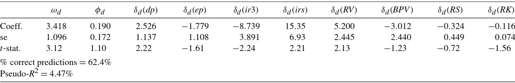
Table 2. Estimation results from the direction model
ωd φd δd(dp) δd(ep) δd(ir3) δd(irs) δd(RV) δd(BPV) δd(RS) δd(RK)
Coeff. 3.418 0.190 2.526 −1.779 −8.739 15.35 5.200 −3.012 −0.324 −0.116
se 1.096 0.172 1.137 1.108 3.891 6.93 2.445 2.440 0.449 0.074
t-stat. 3.12 1.10 2.22 −1.61 −2.24 2.21 2.13 −1.23 −0.72 −1.56
% correct predictions=62.4% Pseudo-R2=4.47%
NOTE: Notes:δd(z)denotes the coefficient on variablez.See notes to Table1for the definition of variables.BPV,RS,andRKstand for bipower variation, realized third moment and realized fourth moment. All predictors are measured at timet−1. The table reports the estimates (along with robust standard errors andt-statistics) for the logit equationpt= exp(θt) /(1+exp(θt))withθt determined by (3), that are obtained from the decomposition model with the Clayton copula. Pseudo-R2denotes the squared correlation coefficient between the observed and predicted probabilities.
macroeconomic predictors are the same as in the linear pre-dictive regression but the combined effect of the two realized volatility measures,RV andBPV, on the direction of the mar-ket is positive. The realized measures of the higher moments of returns do not appear to have a statistically significant effect on the direction of excess returns although they still turn out to be important in the out-of-sample exercise below.
Table3reports the results from the volatility model. The ad-equacy of the Weibull specification is tested using the excess dispersion test based on comparison of the residual variance to the estimated variance of a random variable distributed accord-ing to the scaled Weibull distribution:
ED=√T T −1
t(ηt−1)2−ση2
T−1
t((ηt−1)2−ση2)2
,
whereση2=Ŵ(1+2ς−1)/ Ŵ(1+ς−1)2−1, and hats denote estimated values. Under the null of Weibull specification,EDis distributed as standard normal. Because the excess dispersion test does not reject the null of Weibull density, further general-ization of the density is not needed. On the other hand, the pa-rameterς exhibits statistically significant departures from the value of unity that implies the exponential density.
The high persistence in absolute returns that is evident from our results is well documented in the literature. The nonlinear termρvI[rt−1>0]suggests that positive returns correspond to low-volatility periods and negative returns tend to occur in high volatility periods when the difference in the average volatility of the two regimes is statistically significant. Higher interest rates and earnings-price ratio appear to increase volatility while higher dividend-price ratio and yield spread tend to have the op-posite effect although none of these effects is statistically sig-nificant.
Now we consider the dependence between the two compo-nents—absolute values |rt| and indicators I[rt>0]. The de-pendence between these components is expected to be positive and big, and indeed, from the raw data, the estimated coeffi-cient of unconditional correlation between them equals 0.768. Interestingly, though, after conditioning on the past, the two variables no longer exhibit any dependence. The results for the Frank, Clayton, and FGM copulas are reported in Table4and show that the dependence parameterαis not significantly dif-ferent from zero in any of the copula specifications. Insignif-icance aside, the point estimates are close to zero and imply near independence. The insignificance of the dependence para-meter is compatible with the estimated conditional correlation between standardized residuals in the two submodels,ψt−1|rt| and p−t 1I[rt >0], which is another indicator of dependence. These conditional correlations are close to zero and are statisti-cally insignificant. The result on conditional weak dependence, if any, between the components is quite surprising: once the absolute values and indicators are appropriately modeled con-ditionally on the past, the uncertainties left in both are statis-tically unrelated to each other. Furthermore, the fact of (near) independence is somewhat relieving because it facilitates the computation of the conditional mean of future returns: as dis-cussed in Section2.4, under conditional independence (or even conditional uncorrelatedness) between the components there is no need to compute the most effort-consuming ingredient, the numerical integral (7). For illustration, however, we report later the results obtained when the conditional dependence is shut down, or equivalently,αis set to zero (ignoring dependence), and when no independence is presumed using the estimated value ofαfrom the full model (exploiting dependence).
Table4 also reports the values of mean log-likelihood and pseudo-R2 goodness-of-fit measure. The log-likelihood values
Table 3. Estimation results from the volatility model
ωv βv γv ρv δv(dp) δv(ep) δv(ir3) δv(irs) ς
Coeff. −0.504 0.808 0.035 −0.173 −0.077 0.065 0.348 −0.664 1.275
se 0.244 0.074 0.013 0.059 0.079 0.078 0.344 0.695 0.054
t-stat. −2.07 10.9 2.69 −2.87 −0.98 0.83 1.01 −0.96 5.07
Excess dispersion (ED) test statistic= −0.08 Pseudo-R2=8.58%
NOTE: δv(z)denotes the coefficient on variablez.See notes to Table1for the definition of variables. All predictors are measured at timet−1. The table reports the estimates (along with robust standard errors andt-statistics) for the MEM volatility equation|rt−c| =ψtηt,whereψtfollows (2) andηtis distributed as scaled Weibull with shape parameterς,that are obtained from the decomposition model with the Clayton copula. Thet-statistic in the column forςis computed for the restrictionς=1.The excess dispersion statisticEDis distributed as standard normal with a (right-tail) 5% critical value of 1.65 under the null of Weibull distribution. Pseudo-R2denotes the squared correlation coefficient between the actual and predicted absolute returns.
Table 4. Estimates and summary statistics from copula specifications
Unconditional correlation
Dependence parameterα
Conditional correlation
Coeff. se t-stat. LogL LR Pseudo-R2
Frank copula 0.768 0.245 0.297 0.824 −0.026 1.8404 75.8 7.71%
(0.039)
Clayton copula 0.768 0.087 0.055 1.583 −0.027 1.8422 76.4 7.71%
(0.040)
FGM copula 0.768 0.123 0.149 0.825 −0.026 1.8405 75.9 7.71%
(0.039)
NOTE: “Unconditional correlation” refers to the sample correlation coefficients between|rt−c|andI[rt>c]. “Conditional correlation” refers to the sample correlation coefficients betweenψ−t1|rt−c|andpt−1I[rt>c]estimated from the decomposition model, with robust standard errors in parentheses.LogLdenotes a sample mean log-likelihood value.LRstands for a likelihood ratio test of joint significance of all predictors; its null distribution isχ162 whose 5% critical value is 26.3. Pseudo-R2denotes squared correlation coefficients between excess returns and their in-sample predictions.
for the different copula specifications are of similar magnitude with a slight edge for the Clayton copula which holds also in terms oft-ratios of the dependence parameter. TheLRtest for joint significance of the predictor variables strongly rejects the null using the asymptoticχ2approximation with 16 degrees of freedom. The pseudo-R2goodness-of-fit measure is computed as the squared correlation coefficient between the actual and fit-ted excess returns from different copula specifications. A rough comparison with theR2 from the predictive regression in Ta-ble1 indicates an economically large improvement in the in-sample performance of the decomposition model over the linear predictive regression.
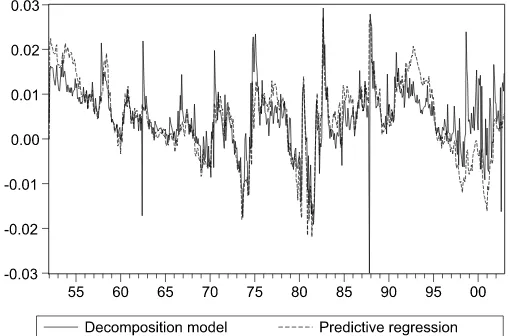
Furthermore, the dynamics of the fitted returns point to some interesting differences across the models. Figure1plots the in-sample predicted returns from our model and the predictive re-gression. We see that the decomposition model is able to predict large volatility movements which is not the case for the predic-tive regression. Moreover, there are substantial differences in the predicted returns in the beginning of the sample and espe-cially post-1990. For instance, in the late 1990s the linear re-gression predicts consistently negative returns while the decom-position model (more precisely, the direction model) generates positive predictions. A closer inspection of the fitted models reveals that most of the variation of returns in the linear regres-sion is generated by the macroeconomic predictors whereas the
Figure 1. Predicted (in-sample) returns from decomposition model and predictive regression.
predicted variation of returns in the direction model is domi-nated by the realized volatility measures. This observation on the differential role of the predictors in the two specifications may have important implications for directional forecasting of asset returns which is an integral part of many investment strate-gies.
3.4 Out-of-Sample Forecasting Results
While there is some consensus in the finance literature on a certain degree of in-sample predictability of excess returns (Cochrane2005), the evidence on out-of-sample predictability is mixed. Goyal and Welch (2003) and Welch and Goyal (2008) find that the commonly used predictive regressions would not help an investor to profitably time the market. Campbell and Thompson (2008), however, show that the out-of-sample pre-dictive performance of the models is improved after imposing restrictions on the sign of the estimated coefficients and the eq-uity premium forecast.
In our out-of-sample experiments, we compare the one-step ahead forecasting performance of the decomposition model proposed in this article, predictive regression and unconditional mean (historical average) model. The forecasts are obtained from a rolling sample scheme with a fixed sample sizeR=360. The results are reported using an out-of-sample coefficient of predictive performance OS (Campbell and Thompson 2008) computed as
OS=1−
T
j=T−R+1∂(rj−rj)
T
j=T−R+1∂(rj−rj) ,
where∂(u)=u2if it is based on squared errors and∂(u)= |u|
if it is based on absolute errors,rjis the one-step forecast ofrj from the conditional (decomposition or predictive regression) model and rj denotes the unconditional mean of rj computed from the lastRobservations in the rolling scheme. If the value ofOSis equal to zero, the conditional model and the uncondi-tional mean predict equally well the next period excess return; if
OS<0, the unconditional mean performs better, and ifOS>0, the conditional model dominates.
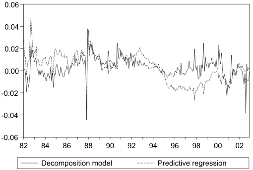
Figure2 plots the one-step ahead forecasts of returns from the predictive regression and the decomposition model with Clayton copula. As in the in-sample analysis, the predicted re-turn series reveal substantial differences between the two mod-els over time. The largest disagreement between the forecasts
Figure 2. Predicted (out-of-sample) returns from decomposition model and predictive regression.
from the two models occurs in the 1990s when the linear re-gression completely misses the bull market by predicting pre-dominantly negative returns while the decomposition model is able to capture the upward trend in the market and the increased volatility in the early 2000s.
Table5presents the results from the out-of-sample forecast evaluation. As in Welch and Goyal (2008) and Campbell and Thompson (2008), we find that the historical average performs better out-of-sample than the conditional linear model and the difference in the relative forecasting performance is around 5%. The predictive regression augmented with the termsI[rt−1>0] andRVt−1I[rt−1>0]appears to close this gap (theOS coef-ficient based on absolute errors is −3.8%) but accounting for nonlinearities in an additive fashion does not seem sufficient to overcome the forecasting advantages of the historical average.
The results from the decomposition model estimated with the three copulas are reported separately for the cases of ig-noring dependence and exploiting dependence. In all speci-fications, our model dominates the unconditional mean fore-cast with forefore-cast gains of 1.33÷2.42% for absolute errors and 1.80÷2.64% for squared errors. Although these forecast gains do not seem statistically large, Campbell and Thompson (2008) argue that a 1% increase in the out-of-sample statistic
OS implies economically large increases in portfolio returns. This forecasting superiority over the unconditional mean
fore-cast is even further reinforced by the fact that our model is more heavily parameterized compared to the benchmark model.
The results from the decomposition model when ignoring and exploiting dependence reveal little difference although the specification withα=0 appears to dominate in the case with absolute forecast errors and is outperformed by the full model in the case of squared losses. Interestingly, the Clayton cop-ula does not show best out-of-sample performance among the three copulas, even though it fares best in-sample. Nonetheless, we will only report the findings using the Clayton copula in the decomposition model in all empirical experiments in the re-mainder of the paper; the other two choices of copulas deliver similar results.
It is well documented that the performance of the predic-tive regression deteriorates in the post-1990 period (Goyal and Welch2003; Campbell and Yogo2006; Timmermann 2008). To see if the decomposition model suffers from a similar fore-cast breakdown, we report separately the latest sample period January 1995–December 2002. TheOSstatistics for this period are presented in the bottom part of Table5. The forecasts from the linear model are highly inaccurate as the decreasing valua-tion ratios predict negative returns while the actual stock index continues to soar. In contrast, the forecast performance of the decomposition model tends to be rather stable over time even though it uses the same set of macroeconomic predictors.
To gain some intuition about the source of the forecasting im-provements, we considered two nested versions of our model: one that contains only the own dynamics of the indicators and absolute returns, and a model that includes only macroeco-nomic predictors and realized measures without any autoregres-sive structure (the results are not reported to preserve space). Interestingly, the forecasting gains of the full model appear to have been generated by the information contained in the predic-tors and not in the dynamic behavior of the sign and volatility components. While the pure dynamic model is outperformed by the structural specification, it still dominates the linear pre-dictive regression and the deterioration in its forecasting perfor-mance appears to be due to poor sign predictability that arises from the weak persistence in the indicator variable mentioned above.
Test of Predictive Ability. To determine the statistical sig-nificance of the differences in the out-of-sample performance of the decomposition model, predictive regression and historical average reported in Table5, we adopt Giacomini and White’s
Table 5. Results from the out-of sample forecasting experiment
Ignoring dependence Exploiting dependence
Linear model Frank Clayton FGM Frank Clayton FGM
1982:01–2002:12
Squared errors −4.62 2.06 1.92 1.80 2.64 2.50 2.56
Absolute errors −4.81 2.42 2.21 2.21 1.54 1.33 1.40
1995:01–2002:12
Squared errors −21.43 2.21 1.82 1.52 2.07 1.59 1.85
Absolute errors −15.84 0.88 0.43 0.36 −0.86 −1.34 −1.21
NOTE: Shown are values of theOSstatistic (in %). The rolling scheme uses a sample of fixed sizeR=360. “Ignoring dependence” means that the decomposition model is estimated but predictions are constructed under the presumption of conditional independence between signs and absolute returns. “Exploiting dependence” means that the decomposition model is estimated and fully used in constructing predictions by (5), including numerical integration.
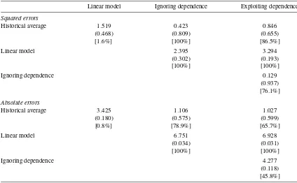
Table 6. Results of the test of predictive ability
Linear model Ignoring dependence Exploiting dependence
Squared errors
Historical average 1.519 0.423 0.846
(0.468) (0.809) (0.655)
[1.6%] [100%] [86.5%]
Linear model 2.395 3.294
(0.302) (0.193)
[100%] [100%]
Ignoring dependence 0.129
(0.937) [76.1%]
Absolute errors
Historical average 3.425 1.106 1.027
(0.180) (0.575) (0.599)
[0.8%] [78.9%] [65.7%]
Linear model 6.751 6.928
(0.034) (0.031)
[100%] [100%]
Ignoring dependence 4.277
(0.118) [45.8%]
NOTE: Top entries in each cell are the values of the test statistic ofH0:E(ht△Lt+1)=0 for modelsiandjin rowiand columnj, respectively, withht=(1,△Lt)′. The null distribution of the test isχ22and the correspondingp-values are in parentheses. The entries in square brackets indicate the percentage of time the model in columnjdominates the model in rowi.
(2006) conditional predictive ability framework. Let△Lt+1 de-note the difference of the loss functions (quadratic or absolute losses) of two models (for example, the predictive regression and the decomposition model) at time t+1. Then, the null of equal predictive ability of two models can be expressed as
H0:Et(△Lt+1)=0 orH0:E(ht△Lt+1)=0, wherehtis aq×1 vector that belongs to the information set at timet. The test of equal predictive ability is based on a (weighted) quadratic form of the sample analog ofE(ht△Lt+1)and isχq2-distributed un-der the null. For details, see Giacomini and White (2006).
Table6presents the values of the test statistic of equal con-ditional predictive ability of two models along with the cor-responding p-values and the percentage of time the model in column j (j=1,2,3) is preferred over the model in row i
(i=1,2,3). The tests computed from the squared errors do not reveal any statistically significant differences across the mod-els although the percentage indicators for the relative perfor-mance of the models suggest that the decomposition model dominates both the historical average and predictive regression,
and the historical average in turn outperforms the linear model. The test based on the absolute errors, however, provides con-vincing statistical evidence of superior predictive performance of the decomposition model and the historical average over the predictive regression. The differences between the decomposi-tion model and the historical average are not statistically sig-nificant although the percentages for the relative performance of the models again indicate some out-of-sample superiority of the decomposition model. Consistent with the results in Table5, exploiting dependence between the two components appears to offer some advantages in terms of squared forecast errors but not in terms of absolute losses.
Mincer–Zarnowitz Regressions. Another convenient ap-proach to evaluating forecasts from competing models is the Mincer–Zarnowitz regression (Mincer and Zarnowitz 1969). The Mincer–Zarnowitz regression has the form
rt=a0+a1rt+error
fort=R+1, . . . ,T, wherert is the actual return andrt is the predicted return. Table7reports the estimates andR2’s from the
Table 7. Results from the Mincer–Zarnowitz regression
Historical average Linear model Ignoring dependence Exploiting dependence
a0 0.046 0.005 0.000 0.003
(0.014) (0.003) (0.003) (0.003)
a1 −11.72 0.208 0.630 0.721
(3.96) (0.223) (0.228) (0.268)
p-value 0.002 0.001 0.180 0.450
R2 2.8% 0.4% 2.5% 2.4%
NOTE: The Mincer–Zarnowitz regression isrt=a0+a1rt+errorfort=R+1, . . . ,T. Heteroscedasticity-robust standard errors are in parentheses. The last two rows report the p-value of the Wald test fora0=0 anda1=1 and the regressionR2.
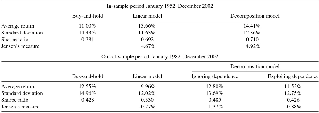
Table 8. Summary statistics of different trading strategies in-sample and out-of-sample
In-sample period January 1952–December 2002
Buy-and-hold Linear model Decomposition model
Average return 11.00% 13.66% 14.41%
Standard deviation 14.43% 11.63% 12.36%
Sharpe ratio 0.381 0.692 0.710
Jensen’s measure 4.67% 4.92%
Out-of-sample period January 1982–December 2002
Decomposition model
Buy-and-hold Linear model Ignoring dependence Exploiting dependence
Average return 12.55% 9.96% 12.80% 11.53%
Standard deviation 14.96% 12.02% 13.69% 12.75%
Sharpe ratio 0.428 0.330 0.485 0.426
Jensen’s measure −0.27% 1.37% 0.88%
NOTE: Reported are annualized average returns and standard deviations. The Sharpe ratio is computed as the average excess return on the portfolio divided by its standard deviation. Jensen’s measure or alpha is obtained as [portfolio excess return−portfolio beta·excess market return].
Mincer–Zarnowitz regressions for the different models along with the Wald test of unbiasedness of the forecastH0:a0=0, a1=1.
The Mincer–Zarnowitz regression results in Table 7 reveal some interesting features of the forecasts from the competing models. Despite its relatively good performance in terms of symmetric forecast errors, the historical average forecasts prove to be severely biased. This seemingly conflicting performance of the historical average can be reconciled by the fact that the near-zero values of the historical average and its low variabil-ity produce OSstatistics that are practically indistinguishable for a wide range of parameters in the Mincer–Zarnowitz regres-sion. The forecasts from the predictive regressions also tend to be biased and the unbiasedness hypothesis is overwhelmingly rejected. None of the copula specifications reject the null of
a0=0 anda1=1 and their forecasts, especially the forecasts from the decomposition model exploiting dependence, appear to possess very appealing properties.
3.5 Economic Significance of Return Predictability: Profit-Based Evaluation
In order to assess the economic importance of our results, we use a profit rule for timing the market based on forecasts from different models. More specifically, we evaluate the model fore-casts in terms of the profits from a trading strategy for active portfolio allocation between stocks and bonds as in Breen et al. (1989), Pesaran and Timmermann (1995), and Guo (2006), among others. The trading strategy consists of investing in stocks if the predicted excess return is positive or investing in bonds if the predicted excess return is negative. Note that these investment strategies require information only about the future direction (sign) of returns although the indicator forecasts are obtained from the estimation of the full model. The initial in-vestment is $100 and the value of the portfolio is recalculated and reinvested every period.
To make the profit exercise more realistic, we introduce pro-portional transaction costs of 0.25% of the portfolio value when the investor rebalances the portfolio between stock and bonds
(Guo2006). The profits from this trading strategy are computed from actual stock return and risk-free rate after accounting for transaction costs and are compared to the benchmark buy-and-hold strategy.
We first look at the performance of the portfolios constructed from the decomposition and linear regression model using in-sample predicted returns. The values of the portfolios at the end of the sample are $20,747 for the buy-and-hold strategy, $62,516 from the trading strategy based on the predictive re-gression, and $80,430 from the decomposition-based trading rule. Table8reports some summary statistics of the different in-vestment strategies such as average annualized return, standard deviation, Sharpe ratio, and Jensen’s measure (alpha). The cor-responding average annualized returns (standard deviations) for the buy-and-hold, regression-based, and decomposition-based trading rules are 11.00% (14.44%), 13.66% (11.63%), and 14.41% (12.36%) with Sharpe ratios of 0.381, 0.692, and 0.710, respectively.
Now we turn our attention to the more realistic investment strategies based on out-of-sample predictions. The setup is the same as in the previous section when the model is estimated from a rolling sample of 360 observations and is used to pro-duce 252 one-step ahead forecasts of excess returns. The results are reported in the second panel of Table8. While the out-of-sample performance of the decomposition model is not as im-pressive as the in-sample exercise, they still provide strong ev-idence for the economic relevance of our approach. It is worth stressing that the out-of-sample period that we examine (Janu-ary 1982–December 2002) coincides with arguably one of the greatest bull markets in history, which explains the excellent performance of the buy-and-hold strategy (average annualized return of 12.55%). It is also interesting to note that the historical average forecasts give rise to a trading strategy that is equivalent to the buy-and-hold strategy since all forecasts are positive.
Despite the favorable setup for the buy-and-hold strategy, the trading strategy based on the decomposition model produces similar returns, 12.8% under independence and 11.53% with dependence, but accompanied with a large reduction in the port-folio standard deviation from 14.96% to 13.69% for the model
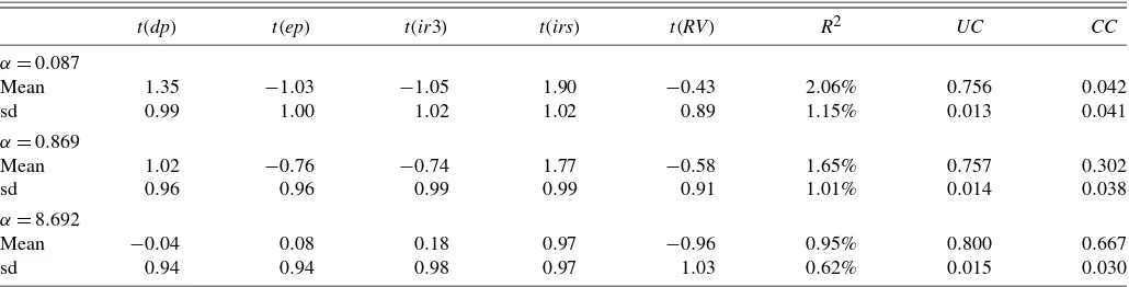
Table 9. Average statistics of predictive regressions run on simulated samples
t(dp) t(ep) t(ir3) t(irs) t(RV) R2 UC CC
α=0.087
Mean 1.35 −1.03 −1.05 1.90 −0.43 2.06% 0.756 0.042
sd 0.99 1.00 1.02 1.02 0.89 1.15% 0.013 0.041
α=0.869
Mean 1.02 −0.76 −0.74 1.77 −0.58 1.65% 0.757 0.302
sd 0.96 0.96 0.99 0.99 0.91 1.01% 0.014 0.038
α=8.692
Mean −0.04 0.08 0.18 0.97 −0.96 0.95% 0.800 0.667
sd 0.94 0.94 0.98 0.97 1.03 0.62% 0.015 0.030
NOTE: Shown are averaget-statistics,R2, unconditional and conditional correlations, together with their standard deviations (sd), from predictive regressions run on 10,000 artificial samples calibrated to the estimated decomposition model with Clayton copula. See notes to Table1for the meaning oft(·)and definitions of variables. All predictors are measured at timet−1.UCandCCdenote the unconditional and conditional, respectively, correlation coefficient between the two components of simulated returns.
under independence and to 12.75% for the full copula speci-fication. As a result, the portfolio based on the independence specification has a Sharpe ratio of 0.485 (versus 0.428 for the market portfolio) and 1.37% risk-adjusted return measured by Jensen’s alpha. In sharp contrast, the portfolio constructed from the linear predictive regression has a Sharpe ratio of 0.330 (av-erage annualized return 9.96% and standard deviation 12.02%) and negative Jensen’s alpha. As before, considering only the 1995–2002 period (results are not reported due to space limita-tions) leads to a significant deterioration of the statistics for the predictive regression whereas the performance of the decompo-sition model is practically unchanged.
3.6 Simulation Experiment
In this section, we conduct a small simulation experiment that evaluates the performance of the predictive regression when the data are generated from the decomposition model pro-posed in the paper. We do this for several reasons. First, it is in-teresting to see if this strategy can replicate the empirical find-ings of relatively strong predictability in the sign and volatility components of returns individually and the weak predictability of returns themselves in a linear framework. This can also help us gain intuition about the importance of the nonlinearities im-plicit in the data generation process but not exim-plicitly picked up by the linear predictive regression. Finally, it is instructive to investigate the effect of different degrees of dependence be-tween the individual components on detecting predictability in the linear specification.
The simulation setup is the following. We generate 10,000 artificial samples from a DGP calibrated to the estimated de-composition model with Clayton copula from Section 3.3, setting the predictor variables to their actual values in the sample. For each artificial sample, we draw an iid series ηt distributed scaled Weibull and an iid seriesνt distributed stan-dard uniform. The estimated volatility model is used to gen-erate the paths of conditional means of absolute returns ψt, which is then transformed into a series of absolute returns by
|rt| =ψtηt. The estimated direction model is used to obtain the processθt, which is subsequently transformed into a series of conditional success probabilitiespt. Next, we compute the se-ries of̺t implied by the Clayton copula and Weibull distribu-tion condidistribu-tional on the series of|rt|,ψt, andpt, and generate a
series of binary outcomesI[rt>0], each distributed Bernoulli with success probability ̺t, by setting I[rt>0] =I[νt< ̺t]. Finally, we construct a sequence of simulated returns using
rt=(2I[rt>0] −1)|rt|. A visual inspection of paths of simu-lated returns indicates that they do not exhibit unexpected (e.g., explosive) patterns.
Table9contains results from the linear predictive regression on simulated data generated using different values of the depen-dence parameterα. The upper panel corresponds to the value of the copula parameterαestimated from the data that implies weak conditional dependence between components (we have also run an experiment with a tiny, nearly zero, value ofα, and obtained very similar measures except, naturally, for the CC
coefficient). The two lower panels correspond to tenfold and hundredfold values of suchαimplying strong and very strong conditional dependence. In all cases the average unconditional correlation between the components is high and approximately matches the value 0.768 in the data, but the average conditional correlation increases substantially asαincreases.
Two remarkable facts pertaining to the predictive regres-sions from Table 9 are worth stressing. The first is that the average t-statistics and R2 in the upper panel are low with even smaller values than we find in the data. This indicates that the linear predictive framework has difficulties detect-ing the predictability in the components even for low degrees of dependence between the components. Adding the terms
I[rt−1>0]and RVt−1I[rt−1>0] as in Table1 increases the R2from 2.06% to 2.58% with averaget-statistics for theRVt−1 and RVt−1I[rt−1>0] terms of−1.14 and 1.29, respectively, while all the other statistics remain very similar. Moreover, and somewhat surprisingly, the averaget-statistics andR2 get even smaller when the dependence between the components in-creases. This is perhaps due to the fact that the greater degree of dependence between the components increases the nonlineari-ties implicit in the multiplicative model and further obscures the relationship between the returns and the predictors in the linear framework. Overall, these results suggest that the linear approximation is unable to capture the predictive content of the multiplicative model.
4. CONCLUSION
This paper proposes a new method for analyzing the dy-namics of excess returns by modeling the joint distribution of