Full Terms & Conditions of access and use can be found at
http://www.tandfonline.com/action/journalInformation?journalCode=ubes20
Download by: [Universitas Maritim Raja Ali Haji] Date: 11 January 2016, At: 23:13
Journal of Business & Economic Statistics
ISSN: 0735-0015 (Print) 1537-2707 (Online) Journal homepage: http://www.tandfonline.com/loi/ubes20
Estimating Intertemporal and Intratemporal
Substitutions When Both Income and Substitution
Effects Are Present: The Role of Durable Goods
Michal Pakoš
To cite this article: Michal Pakoš (2011) Estimating Intertemporal and Intratemporal
Substitutions When Both Income and Substitution Effects Are Present: The Role of Durable Goods, Journal of Business & Economic Statistics, 29:3, 439-454, DOI: 10.1198/jbes.2009.07046
To link to this article: http://dx.doi.org/10.1198/jbes.2009.07046
Published online: 01 Jan 2012.
Submit your article to this journal
Article views: 154
Estimating Intertemporal and Intratemporal
Substitutions When Both Income and
Substitution Effects Are Present:
The Role of Durable Goods
Michal PAKOŠ
Center for Economic & Graduate Education, Department of Economics, Charles University Economics Institute, Academy of Sciences of the Czech Republic, Politickych Veznu 7, 111 21 Prague 1, Czech Republic
(michal.pakos@cerge-ei.cz)
Homotheticity induces a dramatic statistical bias in the estimates of the intratemporal and intertemporal substitutions. I find potent support in favor of nonhomotheticity in aggregate consumption data, with non-durable goods being necessities and non-durable goods luxuries. I obtain the intertemporal substitutability neg-ligible (0.04), a magnitude close to Hall’s (1988) original estimate, and the intratemporal substitutability between nondurable goods and service flow from the stock of durable goods small as well (0.18). Despite that, due to the secular decline of the rental cost, the budget share of durable goods appears trendless.
KEY WORDS: Durable goods; Intertemporal substitution; Intratemporal substitution; Nonhomothetic-ity.
1. INTRODUCTION
The elasticities of intertemporal (across time) and intratem-poral (within period and across goods) substitutions are the two central parameter inputs into all modern macroeconomic mod-els. They dramatically influence the quantitative implications of various economic policy decisions (Hall1988). First, the de-gree of the intertemporal substitutability is by far the most im-portant determinant of the response of saving and consumption to predictable changes in the real interest rate. If expectations of real interest rates shift, there ought to be a corresponding shift in therateof change of consumption expenditures, and hence the amount of consumption itself. The magnitude of this intertemporal substitutability, denoted EIS, is measured by the percentage response of the total consumption expenditures to a percentage change in the real interest rate expectations, ceteris paribus.
Furthermore, in a two-good economy with consumer durable goods, and, more generally, in multigood economies, the mag-nitude of the intratemporal substitution indirectly affects the measure of the intertemporal substitution. A commonly ad-vanced but fallacious argument is that the real interest rate pos-itively affects the user cost of consumer durables, and therefore a surge in interest rates leads to an increase in the user cost, with consumers rationally substituting from the service flow yielded by the durable goods to nondurable consumption. However, in-tertemporal substitutability is a ceteris paribus measure, and it is straightforward to show that as long as the consumption index over the nondurable goods and the service flow from durable goods is homogeneous of degree one, intratemporal substi-tutability doesnotaffect intertemporal substitutability. The sit-uation, however, is diametrically opposite in the case of nonho-motheticity (nonhomogeneous consumption index) wherein the Engel’s income expansion paths are nonlinear functions.
Second, the magnitude of the elasticity of intratemporal sub-stitution may be important for asset pricing. It, in addition to
the coefficient of risk aversion, determines the variability of the marginal utility and hence asset risk premia. In fact, low substi-tutability between consumption goods means that a small vari-ation in nondurable consumption translates into dramatic fluc-tuations in marginal utility. This raises the intriguing question whether the consumption risk of the stock market is really as small as the single-good economies seem to imply.
A large literature focuses on the estimation of these two parameters. In his provocative paper, Hall presents estimates of the elasticity of the intertemporal substitution “. . . that are small. Most of them are also quite precise, supporting the strong conclusion that the elasticity is unlikely to be much above 0.1, and may well be zero.” Using improved inference methods, Hansen and Singleton (1983) find that there is less precision and even obtain estimates that are negative. Using international data, Campbell (1999) estimates the elasticity of intertemporal substitution statistically and economically insignificant. How-ever, these studies assume that the felicity function is separable over nondurables and durables (see Lewbel 1987for another criticism of Hall’s model). In response, Mankiw (1982,1985) and Ogaki and Reinhart (1998) enrich the model by explicitly introducing the service flow from consumer durables but unfor-tunately assume linear Engel curves. Mankiw finds that the ser-vice flow from consumer durables is itself more responsive to the interest rates, and estimates a large elasticity of substitution for durable goods. Focusing on nonseparability across goods, Ogaki and Reinhart find that there is quite a large intertempo-ral substitutability when both nondurable and durable goods are considered.
One important criticism of the Ogaki and Reinhart’s empir-ical results is that they work with homothetic preferences and
© 2011American Statistical Association Journal of Business & Economic Statistics July 2011, Vol. 29, No. 3 DOI:10.1198/jbes.2009.07046
439
Figure 1. Historical consumption series and their relative price. Notes: The plot portrays the time-series of the real nondurable con-sumption (solid line), the stock of durable goods (dashed line), and their relative price (dash–dot line). Bars represent NBER recessions. Sample size 1951:I–2001:IV.
thus their relative demand function for durable goods is free from potentially significant income effects. The correct model-ing of nonhomotheticity in such relative demand turns out to be essential in order to obtain unbiased estimates of the magni-tudes of the intratemporal and intertemporal substitutions. Em-pirically, the ratio of durables over nondurables has been trend-ing up secularly (see Figure1). The mainstream interpretation is that investors optimally substituted (in the sense of Hicks) con-sumer durables for nondurable goods in response to their falling price, with income effects playing no role whatsoever (Eichen-baum and Hansen1990; Ogaki and Reinhart1998). However, durable goods may not have an easy substitute, and therefore we would expect a priori the Hicksian price effects to be rel-atively small. I illustrate this point with an example. Suppose the consumer faces the choice of commuting to work by either taxi or by renting a car. If the car rental cost increases relative to the cost of taxi, the consumer gets a compensation in order to hold his real income constant, and he alters his consumption of car services little relative to the taxi, the Hicksian price effect is small. Note that it is important to compensate the consumer so that we isolate the pure price effect. It is common to use the word “substitute” in the sense of “serving in place of another” (Oxford Dictionary). However, that is not the technical meaning of the word. It confuses income versus substitution effects pre-cisely because in both cases consumers use another consump-tion good in place of the original one. But these two effects are distinct reaction channels to a price change. The presented em-pirical results appear to indicate that the Hicksian substitution effects are smaller than we thought, and thus the income effects should be very important to fit the relative demand function for durable goods.
In order to see the effects of this misspecification, I use the two-step cointegration-Euler equation approach pioneered by Cooley and Ogaki (1996) and Ogaki and Reinhart (1998), and allow for (i) nonseparability across goods (nondurables and the service flow from consumer durables) and (ii) a fairly general form (in fact, my proposed preference specification allows for
time-varying expenditureelasticities of nondurable goods and the service flow from consumer durables as long as their ra-tio is a constant) of nonhomotheticity in the relative demand function for durables by generalizing the constant-elasticity-of-substitution (CES) felicity function. In the first step, using coin-tegration techniques, I obtain super-consistent estimates of the elasticity of intratemporal substitution and the ratio of within-period expenditure elasticities. In the second step, I invoke the Hansen’s (1982) Generalized Method of Moments to effi-ciently estimate the rest of the preference parameter vector, and formally test the model. Then, following Atkeson and Ogaki (1996), I define the elasticity of intertemporal substitution EIS as the inverse of the elasticity of the marginal utility of the total consumption expenditures. This step requires a numerical solu-tion of the second stage of two-stage budgeting to construct the indirect felicity function and its partial derivatives.
The results of the paper are intriguing. First, consistent with microeconomic studies, I find that the Engel curves are not lin-ear, and hence the preferences exhibit nonhomotheticity, with durable goods being luxury goods and nondurable goods nec-essary goods. Second, the budget share of durable goods is time varying, living between 7.3% and 20.4%. It appears trendless, despite the corresponding income elasticity being greater than one, precisely as the rental cost of durables trends down sec-ularly. Hall estimates the EIS for nondurables close to zero whereas Mankiw estimates the EIS for consumer durable goods economically significant. Because the consumption basket is a weighted average of nondurable goods (negligible EIS) and durable goods (significant EIS), and the budget share of durable goods is comparatively small, I confirm the intuitive result that the elasticity of intertemporal substitution EIS for the total con-sumption expenditures is economically small as well.
It is well known that adjustment costs play an essential role in the consumption of durable goods (Bernanke1984; Lam1989; Grossman and Laroque 1990; Eberly 1994). Mankiw (1985) concludes that “. . . future work should pay closer attention to the role of adjustment costs. The model that took account of the adjustment process would be better suited for examining the effects of shorter term fluctuations in the real interest rate.” Ogaki and Reinhart (1998) correctly point out that one of the big advantages of the two-stage cointegration-Euler equations approach is that “. . . it is robust to various specifications of ad-justment costs, relying on the cointegration properties between the observed and the desired stock of durables in the presence of adjustment costs, which is discussed in Caballero (1993).” The inference based on the cointegrating regressions yields con-sistent estimates as long as adjustment costs do not affect the long-run behavior of the service flow from consumer durables. Furthermore, it can be shown that the Euler equation for non-durable consumption is robust to various forms of adjustment costs for durable goods consumption. Unfortunately, many re-lated studies, such as Eichenbaum and Hansen (1990), among others, do not allow implicitly nor explicitly in their estimation for adjustment costs.
2. THEORETICAL FRAMEWORK
2.1 Model
Consider an endowment economy populated with homoge-neous households of measure one. Suppose further that their
preferences are representable by the Von Neuman–Morgenstern time-separable expected utility functional, defined over the stream of consumption{Ct}t≥0. Formally The felicity functionu:R+→R+is of the following isoelastic form
where the parameter σ >0 is a (biased under nonhomoth-eticity) measure of the elasticity of intertemporal substitution (EIS). Next, I specify the consumption indexC:R+×R+→ R+over the nondurable goodsct and the service flowst from
consumer durables as
C(ct,st)
(1− ˜a)×c1t−1/θ+ ˜a×s1t−η/θθ/(θ−1),
wherea˜∈(0,1)is the preference weight. Observe that the con-sumption indexC(ct,st)allows for potentialnonhomotheticity.
Dunn and Singleton (1986) impose that the consumption index
C(ct,st) is homothetic and Cobb–Douglas; their implied
pa-rametersθ=1 andη=1. Eichenbaum and Hansen (1990) and Ogaki and Reinhart (1998) relax the restrictive elasticity con-straint that the intratemporal substitutionθ=1, but still keep the homotheticity postulateη=1. As it will become clear later on, nonhomotheticity, by lifting the assumption of no income effects, turns out to be economically, but also statistically, sig-nificant feature of the data. It markedly improves the fit of the relative demand for consumer durables.
Using the second stage of two-stage budgeting, I interpret the parameterη∈Ras the ratio of within-period expenditure elasticities of nondurables and services flow. Empirically, I find
η <1, and hence durable goods are luxuries and nondurable goods necessities. Homothetic preferences correspond to the restrictionη=1. On the technical side, it is also to be noted that this preference specification easily accommodates variable within-period expenditure elasticities of both goods as long as their ratio remains constant.
Many studies implicitly use durable goods by assuming that nondurable consumption and the service flow from durables enter the felicity function separably (Hansen and Singleton
1982,1983). Eichenbaum and Hansen (1990) find empirical ev-idence in favor of nonseparability. Fleissig, Gallant, and Seater (2000) derive a seminonparametric utility function with both nondurable goods and consumer durable goods, and find that CRRA preferences defined only over nondurable goods are severely misspecified. They also discover evidence in favor of significant nonseparabilities across the consumption goods.
I interpret the parameterθ >0 as a measure of the intratem-poral substitution, which itself is precisely gauged by the elas-ticity of intratemporal substitution, denoted ES. The two, how-ever, are related by the condition derived inAppendix D,ES=
θ+ε∗dd×(η−1), whereε∗ddis the Hicksian own-price elasticity of the demand for the service flow from durable goods. I shall discuss this point deeper hereafter.
The law of motion of the consumer durablesdt is given by
the linear difference equation
dt=(1−δ)dt−1+it,
whereitdenotes durable goods investment, andδ∈(0,1)is the
corresponding depreciation rate. The flow of services st itself
is produced by a linear household production function (Stigler and Becker 1977; Mankiw1985), which is time-independent and state-independent,stA×dt,A>0. The budget constraint
is standard and it is not displayed here.
Note that the preference weighta˜and the household produc-tivity A cannot be separately identified. As a result, I take a monotonic transformation of the utility function, reparametriz-ing the consumption index as
CC(ct,dt)=
ct1−1/θ+adt1−η/θθ/(θ−1), (2.2)
where I denoteaaA˜ 1−η/θ/(1− ˜a) >0.
2.2 First-Order Conditions
The intertemporal marginal rate of substitutionmt+1is given by the ratio the marginal utilities of nondurable goods,
mt+1
My model with nonhomothetic preferences does imply that the intertemporal marginal rate of substitution is stationary de-spite Assumption1.
Assumption 1. The vector time series
[logct,logdt,logqt]′
are integrated of order one, that is,I(1).
Proposition 2. The marginal rate of substitutionmt+1is sta-tionary.
Proof. SeeAppendix B.
Intuitively, mt+1 is the growth rate of the marginal utility βtUc(ct,dt), and if indeed it were integrated of order 1, the
marginal utility would have to be integrated of order 2. Hence, the nonlinear function, the marginal utility, would turn anI(1) variable intoI(2) one, which is impossible.
Standard variational argument implies that the intertemporal first-order condition is the following ubiquitous Euler equation
1=Et[mt+1Rit+1], (2.3)
whereRit+1is the (gross) return on test asseti.
The intratemporal first-order condition states that the marginal utility per last dollar spent must be the same across all consump-tion categories. Formally,
whererctstands for the rental cost of consumer durables. Note
that nondurable goods are the numeraire. Rearranging, we ob-tain the familiar condition that the marginal rate of substitution equals the relative price.
Ud(ct,dt)
Uc(ct,dt)
=rct.
No arbitrage, consequently, links the rental cost of durable goodsrct and their relative “cum-dividend” priceqt by means
of the following present-value formula:
rct=qt−(1−δ)Et{mt+1qt+1}. (2.5) Intuitively, suppose we purchase one unit of durable goods at priceqt, which after one period depreciates to 1−δ. We can
sell it for (1−δ)qt+1. The implicit rental cost rct is the net
present value (NPV) of this transaction, that is,
rct=qt−(1−δ)Et{mt+1qt+1}, (2.6) where the stochastic discount factor just equals the intertempo-ral marginal rate of substitution.
My model implies, under mild conditions, a certain long-run relationship between nondurable consumption, the stock of consumer durable goods, and their relative price. To prove that, I appeal to the well-established fact in empirical macroe-conomics that the asset prices to current income flows, such as price–dividend ratios of common stocks, are stationary, that is,I(0). Durable goods may be thought of as assets that pay a regular stream of rental costs, and hence one naturally conjec-tures that the corresponding price–rental cost ratio ought to be
I(0). That the presented model inherently implies such a long-run relationship is proved in the following proposition.
Proposition 3. The log of the rental cost of durable goods logrctand the log of the durable goods price logqtshare a
com-mon stochastic trend, with the cointegrating vector[1,−1]′.
Proof. SeeAppendix C.
The next proposition turns out to be key in the empirical sec-tion. It allows me to estimate a subset of preference parameters, namely θ and η, superconsistently by applying the Johansen (1991) methodology, and thus immensely simplifies the econo-metric analysis of the model-implied conditional Euler equa-tions by reducing the cardinality of the parameter space.
Proposition 4. The log of nondurable consumption, the log of the stock of durable goods and their relative price share a single common stochastic trend, with the corresponding cointe-grating vector
[1,−η,−θ]′.
Proof. Direct calculation of the intratemporal marginal rate of substitution yields that
Taking natural logarithm of both sides,
log(rct)∝(1/θ )logct−(η/θ )logdt.
Proposition3tells us that
logrct−logqt∼I(0).
Upon substitution, and rearranging, I obtain the claimed long-run relationship
logct−θlogqt−ηlogdt∼I(0).
Evidently, the cointegrating vector is[1,−η,−θ]′. The unique-ness is implied by the fact thatθandηare structural preference parameters.
2.3 Interpretation of the Parametersθ andη
The preference parametersθandηare easily interpreted in the case of deterministic setup using the second stage of two-stage budgeting, which holds due to the weak separability of the consumer preferences (Deaton and Muellbauer 1980). I here summarize the results and refer the interested reader to Ap-pendix Dfor formal derivations.
Each period the consumer optimally chooses his consump-tion expenditureet. Then, depending on the rental cost of
sumer durables, she chooses her allocation of nondurable con-sumption and the service flow from renting consumer durables. The elasticity of intratemporal substitution ES—substitution across goods within a given time-period holding the real in-come constant, gauges how much the relative Hicksian demand for durable goods changes in response to a percent change in the rental cost of consumer durablesrc. In the model, its yard-stick, but not a precise measure, is the parameterθ. The two are related by the equationES=θ+ε∗dd×(η−1), whereε∗ddis the Hicksian own-price elasticity of the demand for the service flow of durable goods. Furthermore, the expenditure elasticity mea-sures how much the demand for a consumption good changes in a response to a 1% rise in expenditures, ceteris paribus. For fu-ture reference, I denote the expendifu-ture elasticity of nondurable consumption ηc and that of the service flow ηd. It turns out
that the parameterηis a ratio of these two elasticities, namely,
η=ηc/ηd. That these claims hold true may be easily verified by
comparing the slopes in the cointegrating regressions based on (i) the intratemporal first-order condition and (ii) the first-order condition from the second stage of two-stage budgeting (D.18), derived inAppendix D.
When both income and substitution effects are present, the relative demand function takes the form
dlog(ct/dt)=ES×dlogrct
+(ηc−ηd)×dlogˆet.
substitution effect income effect
The parametereˆt denotes the real expenditure on both
con-sumption goods, measured in terms of the composite good (see also Appendix D). This equation shows that the relative de-mand changes are either due to substitution effect or due to income effect. It offers a framework to understand the secular rise in the consumption of durable goods relative to nondurable goods. The typical interpretation is that consumers substituted (in the sense of Hicks) to durable goods in response to their falling relative price, with income effects playing no role at all. This corresponds to the case where elasticity of substitu-tion ES is large [Eichenbaum and Hansen’s (1990) estimate is
ES=0.91. Ogaki and Reinhart’s (1998) estimate is greater than one,ES>1] and the preferences are homothetic, which auto-matically eliminates the income effect. Formally,
dlog(ct/dt)=ES×dlogrct. (2.7)
As the empirical results in later sections indicate, after cor-recting for the income effects, the substitutability ES between the services flow and nondurables is smaller than estimated by Eichenbaum and Hansen (1990) and Ogaki and Reinhart (1998), and hence significant nonhomotheticity is dictated. For-mally,(ηc−ηd)×dlogeˆtis not negligible, and thus affects the
estimates of both the intratemporal and intertemporal substitu-tions.
The real income in the United States economy has been rising steadily and thus the previous equation suggests that
ηc−ηd<0. Because the average income elasticity must be
one, we get the plausible result that durable goods are lux-ury goods and nondurable goods are necessary goods, that is,
ηc<1< ηd. Empirically, I estimate ηd∈ [1.460,1.579] and
ηc∈ [0.882,0.954]. For comparison, Costa (2001) estimates
the income elasticities for food at home 0.47 in 1960–1994 and 0.62 in 1917–1935. Those for total food are 0.65 in 1960–1994 and 0.68 in 1917–1935 and in 1888–1917.
3. EMPIRICAL SECTION
3.1 Consumption and Asset Return Data
Quarterly consumption data are from the U.S. national ac-counts as available from the Federal Reserve Bank of St. Louis. I measure nondurable consumptionct as the sum of real
per-sonal consumption expenditures (PCE) on nondurable goods and services. Consumer durables include furniture, motor ve-hicles, and jewelry and watches. The data were kindly provided to me by Motohiro Yogo of Wharton. Note that these time se-ries, after aggregated to annual quantities, areexactly consistent
with the year-end estimates of the chained quantity index for net stock of consumer durables as published by the Bureau of Economic Analysis (BEA). The implied depreciation rate for the durable goods as a whole is approximately 6% per quar-ter. Both nondurable goods and services, and durable goods are converted to per-capita values by dividing by the population size. The relative price of consumer durablesq is calculated as the ratio of the price index for PCE on durable goods to the price index for PCE on nondurable goods and services. The data are available for the period 1951:I–2001:IV.
The asset return data consist of the time series of the monthly return on the U.S. Treasury Bills, and the value-weighted return on all NYSE, AMEX, and NASDAQ stocks (from CRSP), both converted to quarterly values. The real returns are computed by deflating the nominal returns with the consumer price index (CPI), obtained from the Federal Reserve Bank of St. Louis.
3.2 Intratemporal First-Order Condition
Intratemporal First-Order Condition as a Cointegrating Re-gression. As shown in the theoretical section, Proposition4, the intratemporal first-order condition is inherently log-linear,
logct∝θlogqt+ηlogdt+εt
and the disturbace term εt is statistically stationary, that is,
εt∼I(0). Therefore, the model implies a certain single
long-run relationship between nondurable goods, consumer durables, and their relative price. Hence, I am able to estimate the param-etersθ andη superconsistently by extracting the information
from the trends. This idea is borrowed from the related paper by Ogaki and Reinhart (1998), who also estimate the elasticity of intratemporal substitution in the presence of durable goods. They focus on the homothetic case η=1, in which the true elasticity of intratemporal substitutionES=θ. Their regression specification is as follows:
log(ct/dt)∝θlogqt+εt.
The presence of significant nonhomotheticity biases upward the estimate of the intratemporal substitutability. The relative demand for consumer durable goods may change either due to income effect or due to substitution effect. Homotheticity dic-tates that it was Hicksian substitution in response to a secu-lar change in the relative price that led consumers to purchase more durable goods. Neglecting income effects forces the sub-stitution effects to be larger to fit the secular trend in the con-sumption of durable goods relative to nondurable goods. In gen-eral, considering income effects may be important, in particular for goods with large expenditure shares and/or no easy substi-tutes such as housing or consumer durables, as Slutsky equa-tion says that the income effects are proporequa-tional to the expen-diture shares. Empirically, Eichenbaum and Hansen (1990) use CES aggregator over nondurables and durables but impose ho-motheticity. They estimate both intratemporal and intertempo-ral equations jointly using GMM and get the elasticity of in-tratemporal substitutionES=0.91. Using the same preference specification but estimating the elasticity of substitution using cointegration techniques, Ogaki and Reinhart (1998) cannot re-ject the null hypothesisH0:θ≥1. As argued before, neglecting income effects biases upward the estimate of the elasticity of substitution ES, and thus the parameter θ. This observation is confirmed empirically hereafter.
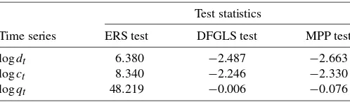
Unit Roots. I test the null hypothesis that the natural loga-rithm of the series, logct, logdt, and logqt, are difference
sta-tionary against the alternative hypothesis of trend stationarity, invoking the efficient unit root tests of Elliott, Rothenberg, and Stock (1996) and Ng and Perron (2001). In all cases, I am un-able to reject the hypothesis that the data are difference station-ary at conventional significance levels (see Table1).
Johansen’s (1991)Cointegration Methodology. Both BIC and HQ criteria suggest that the 3×1 vector
(logct,logdt,logqt)′
follows a vector autoregression of order 2, VAR(2), in levels. The lag lengthpfor the vector error correction model (VECM) is thenp=2−1=1. Since the vector time series are trending,
Table 1. Tests for the null of difference stationarity
Test statistics
Time series ERS test DFGLS test MPP test
logdt 6.380 −2.487 −2.663
logct 8.340 −2.246 −2.330
logqt 48.219 −0.006 −0.076
NOTE: The null hypothesis is that the respective series contain a unit root. The alterna-tive hypothesis is that there is a linear time trend. Tests are as follows: ERS is the Elliott– Rothenberg–Stock test, DFGLS is the DF test with GLS detrending, and MPP is the mod-ified Phillips–Perron test. None of the presented statistics are significant at conventional significance levels.
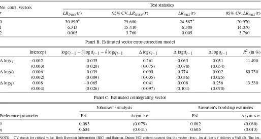
Table 2. Analysis of cointegration
Panel A. Johansen’s likelihood ratio tests
No. coint. vectors r
Test statistics
LRtrace(r) 95% CV,LRtrace(r) LRmax(r) 95% CV,LRmax(r)
0 30.899∗ 29.680 24.587∗ 20.970
1 6.313 15.410 6.308 14.070
2 0.005 3.760 0.005 3.760
Panel B. Estimated vector error-correction model
Intercept logct−1− ˆηlogdt−1− ˆθlogqt−1 logct−1 logdt−1 logqt−1 R2(in %)
logct −0.002 0.035 0.261 −0.063 0.051 11.490
(0.003) (0.020) (0.075) (0.078) (0.054)
logdt −0.006 0.039 0.090 0.774 0.002 80.730
(0.002) (0.009) (0.035) (0.036) (0.025)
logqt 0.008 −0.065 0.041 0.008 0.256 13.530
(0.004) (0.026) (0.097) (0.101) (0.070)
Panel C. Estimated cointegrating vector
Johansen’s analysis Swensen’s bootstrap estimates
Preference parameter Est. Asym. s.e. Est. Asym. s.e.
θ 0.083 (0.075) 0.082 (0.080)
η 0.604 (0.041) 0.605 (0.013)
NOTE: CV stands for critical value. Both Bayesian Information (BIC) and Hannan–Quinn (HQ) criteria suggest that the vector(logct,logdt,logqt)′follows a VAR(2). The
log-likelihood function attains a maximum of 2458.18, with 202 degrees of freedom. Sample period 1951:I–2001:IV. Standard errors are in parentheses.
the Johansen Likelihood Ratio (LR) tests are computed assum-ing unrestricted constant. DenoteH0(r):r=r0the null hypoth-esis of exactlyr0cointegrating vectors, andH1(r):r>r0the al-ternative hypothesis of more thanr0such vectors. Based on Ta-ble2, panel A, I cannot accept the null hypothesisH0(0)at the 5% significance level, but I acceptH0(1).Therefore, according the Johansen’s trace statistic, there is exactly one cointegrating vector. Johansen’s maximum eigenvalue statistic LRmax leads
to exactly the same conclusion, providing an additional support for the single long-run relationship between the logs of non-durable goods, consumer non-durable goods and their relative price.
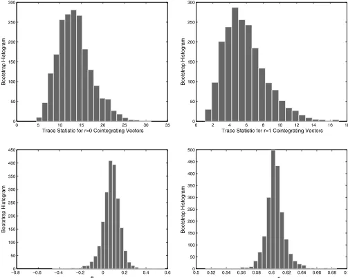
Swensen’s(2006)Bootstrap Algorithm for Determining the Cointegration Rank. It is well known that the asymptotic ap-proximations to the Johansen’s trace and maximum eigenvalue tests are not always accurate. Swensen suggests a bootstrap al-gorithm as an alternative, and I implement it as an important robustness check. Due to their high costs, I perform 2000 ex-periments, and subsequently compute the percentile confidence intervals and p-values for the trace statistic. I easily reject the hypothesis of no-cointegration, with the correspondingp-value being 5e–4. Hence, there is at least one cointegrating vector. I test the null hypothesisH0(1):r=1 versus the alternative of at least two cointegrating vectors. The resultantp-value equals 0.381, and I am unable to reject the null, providing further em-pirical support in favor of a single stochastic trend in the logs of nondurable consumption, the stock of consumer durable goods and their relative price (see also Figure2). Note that this result is essential as the model in fact predicts that these variables are cointegrated, and therefore a failure to find evidence in favor thereof would lead to outright rejection of the model.
Estimated Cointegrating Vector: Johansen Methodology.
I estimate the corresponding vector error correction model by the method of maximum likelihood. The estimates are reported in Table2, panel C. The nonhomotheticity measureη comes economically and statistically less than one, providing evidence against the null hypothesis of homotheticity. The substitutabil-ity yardstickθ is estimated economically small, around 0.08, and statistically less than the estimates of Ogaki and Reinhart (1998). I am able to easily reject the hypothesis that the con-sumption indexC(ct,st)is of the homogeneous Cobb–Douglas
functional form.
Estimated Cointegrating Vector: Swensen Methodology. As a byproduct of bootstrapping the cointegration rank, I obtain es-timates of the empirical distributions for the preference param-etersθandη, which enables me to construct the corresponding bootstrap percentile confidence intervals. Figure2dislays the corresponding histograms. Table2, panel C, presents the re-sults. As may be observed, both methods lead to essentially the same point estimates.
Robustness Check: Failure of Model-Implied Cointegration Under Postulated Homotheticity. The model implies a single long-run relationship between the logs of the nondurable goods, the stock of durable goods, and their relative price. Note that the case of homotheticityη=1 is a nested model. I show here-after that imposing artificially this constraint empirically breaks down this long-run relationship. In detail, both BIC and HQ criteria suggest that the 2×1 vector (logct−logdt,logqt)′
follows a second-order vector autoregressive process, VAR(2). The lag lengthpfor the vector error-correction model (VECM) is thusp=2−1=1. The null hypothesis of zero cointegrat-ing vector against the alternative of at least 1 cannot be ac-cepted at 5% significance level, using both Johansen’s trace
Figure 2. Histograms: Swensen’s bootstrap.Notes: 2000 bootstrap experiments performed in Splus.
statisticLRtraceand the Johansen’s maximum eigenvalue
statis-ticLRmax. In detail,LRtrace(0)=12.81<15.41=95%
criti-cal value, andLRmax(0)=8.36<14.07=95% critical value.
In addition, the extremized log-likelihood function is about 1489.21, dramatically below 2458.18 obtained by not artifi-cially forcing homotheticity on the data.
My model implies a single cointegrating long-run relation-ship. The fact that the empirical evidence in favor thereof is minimal in case of homothetic preferences indicates that arti-ficially imposing the restriction of no income effects upon the relative demand function would lead to an outright rejection of the model.
Overall, it appears fair to conclude that there is an over-whelming evidence in favor of nonhomotheticity in the relative demand function for consumer durables.
Plausible Magnitude of the Parameter a: Implications of the Intratemporal First-Order Condition. Durable goods may be thought of as assets with the priceqt paying a regular stream
of rental costsrct. Note thatqtis the “cum-dividend” price. To
illuminate the analysis, definept=qt−rctas the “ex-dividend”
price. The no-arbitrage condition
rct=qt−(1−δ)Et{mt+1qt+1}
may be expressed equivalently in the form more familiar from empirical finance as
pt=(1−δ)Et{mt+1[pt+1+rct+1]}
or
1=Et{mt+1(1−δ)[pt+1+rct+1]/pt},
where mt+1 plays the role of the stochastic discount factor. The implied rate of return on the durable goods is then evidently
Rdurablest+1 =(1−δ)(pt+1+rct+1)/pt
and we obtain the familiar Euler equation
Et[mt+1Rdurablest+1 ] =1.
In order to make progress in constructing the rental cost of consumer durable goods, I make the following plausible as-sumption.
Assumption 5. The risk premium on the durable goods,
Rdurablest+1 −Rft, is negligible (zero).
The following simple lemma is useful.
Lemma 6. The risk premium on durable goods is given by the formula Proof. Straightforward using the definition of the condi-tional covariance
covt[Xt+1,Yt+1] =Et[Xt+1Yt+1] −Et[Xt+1]Et[Yt+1].
In view of Assumption5and Lemma6, note that the rental cost price ratio satisfies
As shown in the subsection dealing with the Johansen’s coin-tegration methodology, the vector time series [logct,logdt,
logqt]′ follows a cointegrated VAR(2), and hence I estimate
the corresponding vector error-correction model (see Table 2, panel B) to forecast the growth rate in the (log) durable goods price one quarter ahead, and consequently estimate the rental cost of consumer durable goods from the above formula. Em-pirically, it turns out that multivariate and univariate fore-casts [from AR(1)] are practically identical. In addition, I fit GARCH(1,1)model to the log of the durable goods price to model the variation in the conditional second moment. I per-form several diagnostic checks. I test for the ARCH effects in the residuals. Then, I estimate GARCH(1,1) assuming a Gaussian distribution. Quantile-to-quantile plot for standarized residuals rejects this distributional assumption, and so does the Kolmogoroff–Smirnoff test. Hence, I assume that the errors come from thet distribution, the degree of which is also esti-mated. Quantile-to-quantile plot supports this distributional as-sumption. Further results available upon request.
Subsequently, having constructed the rental–cost to price ra-tio from the above formula, I estimate the preference parameter
a>0 from the intratemporal first-order condition
a×d−t η/θ
whereθˆandηˆ are the superconsistent estimates. I find empiri-cally that the parametera≈0.007.
This back-of-the-envelope calculation of the magnitude of the parametera serves as an important check when I estimate the rest of the preference parameter vector(σ, β,a)by the effi-cient method of moments.
3.3 Estimation of the Rest of the Parameter Vector: Euler Equations Approach
Methodology. My approach to the estimation and the in-ference of the rest of the prein-ference parameter vector =
(σ, β,a)∈ R+ ×(0,1)×R+ follows Ogaki and Reinhart (1998). These authors show how to modify the analysis of Hansen and Singleton (1982) to allow for multiple consump-tion goods. The primary testable asset pricing implicaconsump-tions of the model are the set of intertemporal Euler equations
Et[mt+1Ri,t+1] =1, (3.2)
wheremt+1is the intertemporal marginal rate of substitution,
mt+1=
βUc(ct+1,dt+1) Uc(ct,dt)
(3.3)
andRi,t+1is the gross return on an asseti.
In addition, we have the intratemporal first-order condi-tion (2.5). Recall from the previous section that the cointegrat-ing regression yields superconsistent estimates for parameters
θandηbut does not pin down the preference weightathat en-ters the formula (2.5). Therefore, it is essential to include the intratemporal first-order condition in the GMM estimation, that is, to include
Et{Udt/(qtUct)−(rct/qt)} =0, (3.4)
where
rct=qt−(1−δ)Et{mt+1qt+1}.
Letztbe a vector of variables in the consumers’ information set
at timet. Using the components ofztas instruments, I form the
vector-valued function I calibrate the parametersθandηusing the super-consistent estimates obtained by the cointegration approach asθˆ=0.082 andηˆ=0.604. I estimate the rest of the preference parameter vector by the choice of that makes the sample moment conditiongT()close to zero in the sense of minimizing the
quadratic form
whereST is the spectral density matrix at frequency zero,
es-timated using quadratic spectral kernel with automatic band-width selection and VAR(1)prewhitening. I use the two-step version of the efficient GMM (Hansen1982).
In my analysis I consider several instrumental variables. First, I use the lagged nondurable consumption growth rate, the lagged growth rate of the stock of durable goods, and the lagged growth rate in the durables price. These are lagged at least twice
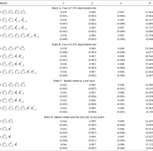
Table 3. GMM results
Instruments σ β a JT
Const,I(t−1)2,It(−1)3,It(2),It(−2)1 0.039 0.988 0.007 28.223 (0.001) (0.002) (0.000) (0.079) Const,I(t−1)2,I(t−1)3,Rft,Rft−1 0.038 0.986 0.007 40.397
(0.001) (0.002) (0.000) (0.000) Const,I(t−2)2,I(t−2)3,Rtf,Rft−1 (0.038) 0.985 0.007 35.515
(0.001) (0.002) (0.000) (0.000) Const,I(t−1)2,It(−1)3,It(−2)2,It(−2)3,Rft,Rft−1 0.038 0.987 0.007 42.643
(0.000) (0.002) (0.000) (0.008)
NOTE: Two-step efficient GMM with the depreciation rate 6% used. The spectral density matrix estimated by means of quadratic spectral kernel with Andrews (1991) automatic bandwith selection and a VAR(1)prewhitening procedure of Andrews and Monahan (1992). The notation for instrument sets is as follows:It(1)= {(Ct/Ct−1), (Dt+1/Dt), (Qt/Qt−1)}, It(2)= {(Ut(1)/U(1)
t−1), (U (2)
t /U(2)t−1)}, whereU (1)
t stands for the number of unemployed less than 5 weeks, andU(2)t stands for the number of unemployed more than 15 weeks. Sample
size 1951:I–2001:IV. HAC standard errors andp-values in parentheses.
to take care of the cash-in-advance constraint inherent in explic-itly monetary models (see also Ogaki and Reinhart1998). Sec-ondly, a natural choice for the instrumental variables are both the growth rate of the number of civilians unemployed less than 5 weeks and the growth rate of the number of civilians unem-ployed more or equal 15 weeks. Finally, I also use the lagged real return on the U.S. Treasury Bills itself as an instrument.
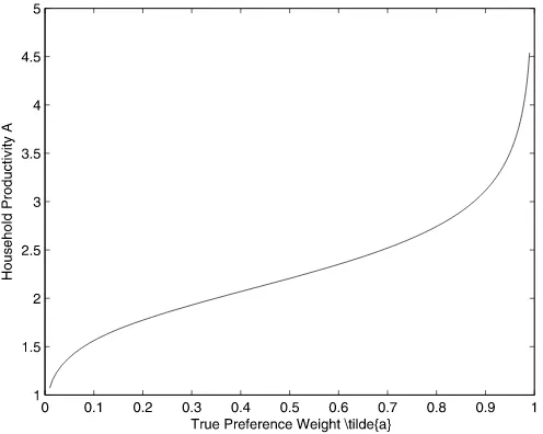
Interpretation of the Empirical Results. Table 3 presents the GMM estimates for four different sets of instruments when the test asset is the U.S. Treasury Bill. The subjective discount factorβ is estimated around 0.986. The estimate is also quite precise, and I am easily able to reject the hypothesisH0:β≥1. The parameter a is estimated to be 0.007. The point esti-mate is also quite precise, with the asymptotic standard error less than 0.001. Note that the point estimate obtained from the efficient method of moments coincides with the back-of-the-envelope calculation based purely on the intratemporal first-order condition as described in a subsection above. Figure 3
plots the combinations of the true preference weighta˜ and the household productivityAwhich are consistent witha=0.007. For example, if the productivity A=1.5, consumer durable goods have about 10% weight in the households’ preferences.
Figure 3. Implied preference weight and household productivity.
The preference parameter σ is estimated from 0.038 up to 0.039, and statistically significant although economically small. Again, the asymptotic standard error is quite small.
The test of the over-identifying restriction statistically rejects the model, except for the first row in Table3. However, it is well known that asymptotic normality may provide a rather poor ap-proximation to the sampling distribution of GMM estimators (Tauchen 1986; Kocherlakota 1990; West and Wilcox 1994; Hansen, Heaton, and Yaron1996). For example, the sampling distribution of GMM estimators can be skewed and can have heavy tails, and tests of overidentifying restrictions can exhibit substantial size distortions. To check the robustness of my re-sults, I follow Hall and Horowitz (1996) who develop a small-sample bootstrap approximations to the distributions of GMM estimators.
Robustness Check: Hall and Horowitz (1996) Bootstrap.
Due to a quite high computational burden, I perform only 1000 bootstrap experiments, focusing only on the last row of Table3. The 95% quantile of the empirical distribution comes about 54.73, which is greater than the corresponding JT statistic of
about 42.64, and hence the model is not statistically rejected. I conclude that the asymptotic Gaussian distribution provides a rather poor approximation to the true sampling distribution of theJT statistic.
Robustness Check: Depreciation Rate of the Durable Goods.
Yogo (2006) in his empirical study carefully constructs the stock of durable goods so that the annual stock equals exactly the estimate of the BEA. He consequently finds that the implied depreciation rate is about, but not exactly, 6%.
I estimate the model assuming the depreciation rate equals 5.5% and 6.5%. The results are presented in Table4, panels A and B, respectively. It is to be noted that the point estimates change minimally from the results in Table3. I therefore con-clude that the statistical analysis is robust to economically rele-vant variation in the depreciation rate.
Robustness Check: Test Assets. As a further robustness check, I also include the real value-weighted return of all NYSE, AMEX, and NASDAQ stocks. Table 4, panel C, presents the GMM estimates when the only test asset is the mar-ket return. The point estimates of the parameter vector(σ, β,a)
are not statistically different from the estimates in Table3. Fi-nally, I include both the three-month Treasury Bill and the mar-ket return. As may be observed from Table4, panel D, the point estimates again do not differ statistically from Table3.
Table 4. GMM: robustness check
Instruments σ β a JT
Panel A. Case of 5.5% depreciation rate
Const,It(−1)2,It(−1)3,It(−2)2,I(t−2)3 0.039 0.989 0.007 27.964 (0.001) (0.002) (0.000) (0.084) Const,It(−1)2,It(−1)3,Rtf−1,Rft−2 0.038 0.986 0.007 40.227
(0.001) (0.002) (0.000) (0.000) Const,It(−2)2,It(−2)3,Rtf−1,Rft−2 0.038 0.984 0.007 35.337
(0.001) (0.003) (0.000) (0.000) Const,It(−1)2,It(−1)3,It(−2)2,It(−2)3,Rft−1,Rft−2 0.038 0.986 0.007 42.328
(0.000) (0.002) (0.000) (0.008)
Panel B. Case of 6.5% depreciation rate
Const,It(−1)2,It(−1)3,It(2),I(t−2)1 0.039 0.989 0.008 28.366 (0.000) (0.002) (0.000) (0.077) Const,It(−1)2,It(−1)3,Rft,Rft−1 0.038 0.987 0.008 40.540
(0.001) (0.002) (0.000) (0.000) Const,It(−2)2,It(−2)3,Rft,Rft−1 0.038 0.985 0.008 35.489
(0.001) (0.002) (0.000) (0.000) Const,It(−1)2,It(−1)3,It(−2)2,It(−2)3,Rft,Rft−1 0.038 0.987 0.008 42.844
(0.000) (0.002) (0.000) (0.007)
Panel C. Market return as a test asset
Const,It(−1)2,It(−1)3,It(−2)2,I(t−2)3 0.042 0.986 0.008 24.080 (0.002) (0.007) (0.001) (0.193) Const,It(−1)2,It(−1)3,Rft,Rft−1 0.044 0.993 0.008 26.055
(0.002) (0.006) (0.001) (0.038) Const,It(−2)2,It(−2)3,Rft,Rft−1 0.043 0.986 0.008 18.038
(0.002) (0.008) (0.001) (0.081) Const,It(−1)2,It(−1)3,It(−2)2,It(−2)3,Rft,Rft−1 0.043 0.989 0.008 29.965
(0.002) (0.006) (0.001) (0.150)
Panel D. Market return and risk-free rate as test assets
Const,It(−1)2,It(−2)2 0.044 0.999 0.008 24.403
(0.003) (0.007) (0.000) (0.059)
Const,It(−1)2,Rtf 0.043 0.996 0.008 29.814
(0.003) (0.007) (0.000) (0.003)
Const,It(−2)2,Rtf 0.045 0.999 0.007 25.927
(0.008) (0.021) (0.000) (0.002)
Const,It(−1)2,It(−2)2,Rft 0.044 0.997 0.008 33.122
(0.003) (0.007) (0.000) (0.016)
NOTE: Depreciation rate 6.0% used in panels C and D. See also notes for Table3.
4. THE BUDGET SHARE, THE RENTAL COST AND THE EXPENDITURE ELASTICITY
OF DURABLE GOODS
Table3, last row, allows me to construct the time series of (i) the implied rental cost of consumer durables rct, (ii) the
budget share of the durable goods expendituressd,t in total
ex-penditureset=ct+rct×dt, and (iii) the nondurables and the
durables expenditure elasticitiesηc,t andηd,t. First, I construct
the implied rental cost of durables as the intratemporal marginal rate of substitution between the service flow from durable goods and nondurable goods,
rct=
Ud(ct,dt)
Uc(ct,dt)
. (4.1)
It is displayed in Figure4, left panel. Empirically, it turns out that the rental cost is between 3.18% to 11.74% of the durable goods price per quarter, depending on the exact date, which appears to be a plausible magnitude. Furthermore, the model implies, and the econometric analysis further confirms that the ratiorct/qtis stationary, and hence both the real rental costrct
and the real durables priceqt decline secularly in the post-war
U.S. economy (see also Figure1). This has an essential impli-cation for the budget share of durable goodssd,t, which in fact
appear trendless, despite the fact that durable goods are luxury goods. Formally, one may easily show by log-differentiating the definition formula for the budget sharesd,tthat
dlogsd,t=(1+εdd,t)×dlogrct+(ηd,t−1)×dloget.
Figure 4. Historical time series of the rental cost of consumer durable goods and the corresponding budget share.Notes: Bars represent NBER recessions. Sample size 1951:I–2001:IV.
Back of the envelope calculation, along with the Slutsky equa-tionεdd,t=ε∗dd,t−sd,t×ηd,t, suggest that indeed the budget
share of durable goods appears trendless over time (see also Figure4, right panel).
In detail, the Marshallian price elasticityεdd,t is small and
negative. First, the Hicksian price elasticityεdd∗,t is small and negative. Durable goods do not have easy substitutes and, in addition, the substitution matrix is negative semidefinite and hence all diagonal terms are nonpositive. Second, all consump-tion goods categories in the model are normal, with expenditure elasticities positive. Third, the budget share of durable goods is relatively small, and, hence, the term(1+εdd,t)≈1. The term
(ηd,t−1)≈0.5, which is less than one. This suggests, and
Fig-ure4 confirms empirically, that despite the nonhomotheticity and the secular increase in the total consumption expenditures (i.e.,dloget>0), the budget share of durable goods appears
trendless precisely because the rental cost of durables declines so steeply, that is,dlogrct≪0, fully offsetting the
correspond-ing income effect.
The intraperiod budget constraint implies that the weighted average of expenditure elasticities must be one
sc,t×ηc,t+sd,t×ηd,t=1, (4.2)
wheresc,t andsd,tare the shares of nondurables and durables,
respectively, in total within-period consumption expenditures
et =ct +rct ×dt. I find that ηd ∈ [1.460,1.579] and ηc ∈
[0.882,0.954]; see also Figure5, bottom two panels. Evidently, durable goods are luxury goods and nondurable goods are nec-essary goods.
5. THE INTRATEMPORAL ELASTICITY OF SUBSTITUTION ES
Although it is tempting to refer to the preference parameterθ
as a yardstick of the intratemporal substitutability, its true mea-sure is given by the relationshipES=θ+εdd∗ ×(η−1), where
εdd∗ is the Hicksian own-price elasticity of the demand for the service flow of durable goods. Figure5, top left panel, portrays the estimated time-series of the elasticity of the intratemporal substitution ES, which lies in the interval of[0.172,0.194].
6. THE INTERTEMPORAL ELASTICITY OF SUBSTITUTION IES
The elasticity of intertemporal substitution IES is an essential input into many dynamic macroeconomic models. Because the preference specification features nonhomotheticity, the elastic-ity of intertemporal substitution EIS does not equal the param-eter σ exactly as is the case under homotheticity. In fact, EIS tells how much the total consumption expenditure, or the sav-ing, if you like, changes in response to predictable changes in the real interest rate.Appendix Eshows that, under determin-istic setup, the intratemporal first-order condition is a solution of the second-stage of two-stage budgeting, and the indirect fe-licity function V(e,rc)is the value function of the following concave program
V(e,rc)= max
{(c,d)∈R2+}
U[C(c,d)] (6.1)
subject to the budget constraint
c+rc×d≤e, (6.2)
whereeis the total consumption expenditure within the period andrcis the rental cost of consumer durables.
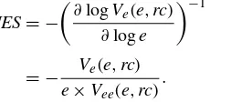
Following Atkeson and Ogaki (1996), I define the intertem-poral elasticity of substitution IES as the inverse of the elasticity of the marginal utilityVe(e,rc)of the total consumption
expen-diturese,
IES= −
∂
logVe(e,rc)
∂loge
−1
(6.3)
= − Ve(e,rc)
e×Vee(e,rc)
. (6.4)
Intuitively, suppose the elasticity of the marginal utilityVe of
the total consumption expenditureseis large. That means that a small change ineleads to a large change in the correspond-ing marginal utilityVe. Because consumers strive to spread their
consumption expenditureseover time, depending on their fore-casts of the real interest rate, in order to maximize their welfare,
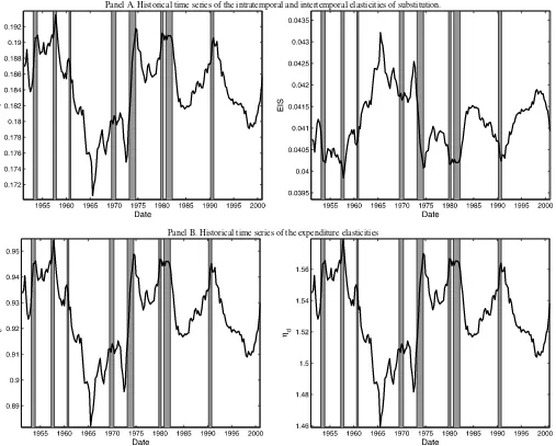
Panel A. Historical time series of the intratemporal and intertemporal elasticities of substitution.
Panel B. Historical time series of the expenditure elasticities
Figure 5. Estimated elasticities.Notes: Bars represent NBER recessions. Sample size 1951:I–2001:IV.
they will alter their spending plans minimally; otherwise, there will be a dramatic variation in marginal utilityVe across time
that cannot be possibly optimal. As a result, the intertemporal elasticity of substitution IES is small and a predictable change in the real interest rate will give occasion to a relatively small change in the consumption expenditurese.
As the preferences are nonhomothetic, a closed-form solu-tion forV(e,rc)may not exist. However, a numerical solution, described inAppendix E, is rather straightforward. See Hanoch (1977) for a different treatment.
Figure5portrays the time-series of the estimated IES for the preference parameter calibrations based on the super-consistent estimates from the intratemporal first-order condition and the GMM estimates from Table3, row 4. As may be observed, the IES is economically negligible.
The economically inconsequential magnitude of the IES for the total consumption expenditures makes intuitive sense. In fact, the budget share of durable goods is only about 7.32%–20.41%. As the bulk of consumption is composed pre-dominantly of nondurable goods with practically zero IES (Hall 1988), it comes as no surprise to discover that consid-ering durable goods that themselves in fact do have high IES
(Mankiw1982) does not raise the overall IES for the total con-sumption. The time-variation in the IES is a direct consequence of the preference nonhomotheticity.
7. CONCLUSION
This paper argues that ignoring the income effects (nonho-motheticity) in the relative demand function for durable goods induces a striking bias in the estimates of the magnitude of the intertemporal and intratemporal substitutions. When I correct for nonhomotheticity, I find the magnitude of the elasticity of intertemporal substitution EIS to be small, on the order of mag-nitude 0.04. In addition, I find compelling evidence against the separability across consumption goods in the felicity function. However, in contrast to Eichenbaum and Hansen’s (1990) value of 0.91 and Ogaki and Reinhart’s (1998) value greater than one, my estimate of the elasticity of intratemporal substitution, after careful correction for nonhomotheticity, is around 0.18. Last, I have found strong evidence in favor of nonhomotheticity in the aggregate consumption data. Nondurable consumption is a nec-essary good and the service flow from durables is a luxury good,
with the within-period expenditure elasticity greater than one. This is consistent with the results in Ogaki (1992) and Costa (2001).
APPENDIX A: IDENTIFICATION AND BACK OF THE ENVELOPE CALCULATION OF THE PLAUSIBLE VALUES OF THE PREFERENCE PARAMETERa
In the empirical part, I reparametrize the consumption index so that all the parameters are identified. For example, we cannot separately identify the preference weighta˜and the coefficientA
from the household production function. In detail, suppose we keep the parametrization of the consumption index as
C(c,d)=(1− ˜a)c1−1/θ+ ˜a(A×d)1−η/θθ/(θ−1). (A.1)
Clearly,a˜∈(0,1)andA∈R+. “Taking out” the number 1− ˜a
from the consumption index, and rearranging the terms yields
C(c,d)=(1− ˜a)θ/(θ−1)
Because applying a strictly increasing operator (i.e., multiply-ing by a positive number in our case) does not change the pref-erence ordering, I may drop the term(1− ˜a)θ/(θ−1). In addition,
the preference specification that I actually use in the GMM es-timation.
There is a deep reason for using this “simpler” consumption index (A.4). In fact, as may be easily inferred from the analysis above, the indices (A.1) and (A.4) are observationally equiva-lent and generate exactly the same preference orderings. How-ever, as econometricians, we clearly cannot separately identify the preference weighta˜and the household production function coefficientA; only the parametera is econometrically identi-fied. Unfortunately, a hurried reader tends to have a strong prior on the plausible magnitudes of the parametera, which seem-ingly looks like a preference weight, and thus wrongly expects magnitudesa∈(0,1).
APPENDIX B: PROOF OF PROPOSITION2
First, in order to work with linear time series, I follow Camp-bell and Shiller (1988), and log-linearize the log of the intertem-poral marginal rate of substitution. In detail, the first-order ap-proximation of the functionF(x)=log[1+exp(x)] around a pointx¯is
F(x)≈F(x)¯ +F′(x)(x¯ − ¯x)
≈log[1+exp(x)¯ ] + exp(x)¯
1+exp(x)¯ (x− ¯x) ∝kx.
As a result, the log offtis approximately
logft≈k
Recall that the (log) intertemporal marginal rate of substition
mt+1is defined as
whereLis the lag, or backshift, operator. According to Assump-tion1, all terms are covariance stationary as they involve growth rates ofI(1) variables.
APPENDIX C: PROOF OF PROPOSITION3
Equilibrium requires a lack of arbitrage in all markets, in-cluding the market for durable goods. The no-arbitrage condi-tion in the goods market is embodied in the following condicondi-tion:
rct=qt−(1−δ)Et[mt+1qt+1]
as explained in the main text. I shall prove the existence of a single long-run relationship between logrct and logqt by
fol-lowing Campbell and Shiller (1988). Note that durable goods price to rental cost is the exact analogue to the price–dividend ratio in the model of common stocks. In detail, rearranging the previous no-arbitrage condition yields
where I assumed in the last step that the time series is Gaussian as not much is known about nonlinear time series.
According to Assumption 1, the log-durable goods price logqt∼I(1), and according to Proposition2 logmt+1∼I(0). Define the 4×1 vector
ξt= [(1−L)logct, (1−L)logdt, (1−L)logqt,logmt]′.
Wold representation theorem (e.g., Brockwell and Davis1991, p. 187) says that the stochastic process ξt has MA(∞) repre-summable matrix series. I assume that the forecast errorsεtare
Gaussian. In addition, I invoke the following simple lemma.
Lemma 7. Let the filtration {Ft}t∈N be defined as Ft =
σ ({cs,ds,qs: 0 ≤ s ≤ t}). Then, the stochastic process
{E(ξt+1|Ft)}t∈Nis a covariance stationary process.
Proof. Direct calculation shows that
In view of this, we have that
log
Finally, log-linearize, following Campbell and Shiller (1988) the relationship log(1−rct
APPENDIX D: INTERPRETATION OF THE PREFERENCE PARAMETERS IN
A DETERMINISTIC SETUP
The preference parameters θ and η are most easily inter-preted in the deterministic setup. Let us think of consumers as renting their stock of durablesdtin a perfect rental market, with
the rental costrctgiven by the right-hand side of equation (2.5),
namely,
rct=qt−(1−δ)Et{mt+1qt+1}. (D.1)
In a deterministic setup, the risk-free interest rate 1+rft =m−t+11
and the rental cost of capital satisfiesrct=qt−(1−δ)(1+
rft)−1qt+1. Viewed this way, the preferences over nondurables and durables are weakly separable. Weak separability is a nec-essary and a sufficient condition for the second-stage of two-stage budgeting to hold (Deaton and Muellbauer 1980). In-tuitively, suppose the consumer has already chosen his opti-mal within-periodttotal consumption expenditureet, expressed
in terms of nondurable consumption, which is a numeraire throughout unless stated otherwise. The level of the nondurable consumptionctand the stock of durable goods to be renteddt
are then chosen so that the second-stage optimization holds, for-mally,
(ct,dt)=arg max
{(˜ct,d˜t)∈R2+}
U[C(c˜t,d˜t)] (D.2)
subject to the budget constraint
˜
ct+rct× ˜dt≤et. (D.3)
Note that the expenditureset in other periodstare unaffected
and the consumer thereby maximizes his lifetime well being. The first-order condition associated with the second stage is helpful to interpret the preference parameters. The Marshallian demands are functions of the relative pricerctand the
expendi-tureet,
The parametersηcandηdare the expenditure elasticities
asso-ciated with the within-periodtexpenditure levelet. They tell us
how much the demandsctanddtchange (in percentage terms)
in response to a 1% rise in the total within-periodt expendi-ture levelet, ceteris paribus. Formally, they are defined as
per-centage changes in the Marshallian demands in response to a percentage change in expenditures, ηc=∂logct/∂loget and
ηd=∂logdt/∂loget. The budget constraint (D.3) implies that
the weighted average of these elasticities must be one. The pa-rameters εcd and εdd are Marshallian price elasticities.
Sub-tracting one equation from the other, using Slutsky equation
εij=εij∗−ηisj, wheresjis the share of goodj∈ {c,d}in
expen-ditureset, andε∗ijis the compensated Hicksian price elasticity,
implies that the relative demand function satisfies
dlog(ct/dt)=ES×dlogrct
+(ηc−ηd)×dlogeˆt, (D.8)
substitution effect income effect
whereES≡ε∗cd−ε∗dd denotes the elasticity of intratemporal substitution (see the discussion below). The variableet is the
expenditure on both consumption goods, expressed in terms of nondurable goods whereas what I call the real expenditureeˆtis
expressed in terms of thecompositegood, with the implicitly defined price index. In fact, it is defined asdlogeˆt=dloget−
sddlogrct. The appropriate price index is pt=1sc×rcstd, and
hence therealexpenditure satisfiesdlogeˆt=dlog(et/pt).
The elasticity of substitution ES is defined as a percentage change in the relative Hicksian demand in response to a per-centage change in the relative price,
ES=∂log(c∗t/d∗t)/∂logrct=εcd∗ −ε
∗
dd (D.9)
and it is a measure of the concavity of the indifference curves. For instance,ES=0 for Leontief preferences and thus the in-difference curves are extremely concave. It may be shown by combining the equations in this appendix that
ES=θ+ε∗dd×(η−1), (D.10) where in anticipation of a future result, I define
θ=(ε∗cd−εdd∗η), (D.11)
η=ηc/ηd. (D.12)
Based on a back of the envelope calculation, the parameter
θ underestimates the true elasticity of intratemporal substitu-tion ES. That is,ε∗ddis nonpositive because the substitution ma-trix is negative semidefinite, and the parameterηis less than one, empirically. As a result,
ES≥θ (D.13)
but I still refer toθas a yardstick of intratemporal substitutabil-ity.
I now derive the deterministic equivalent of the intratemporal first-order condition. Eliminate the expenditureetin the system
of the Marshallian demands to get the conditional demand
dlogct=(ε∗cd−ε