Full Terms & Conditions of access and use can be found at
http://www.tandfonline.com/action/journalInformation?journalCode=ubes20
Download by: [Universitas Maritim Raja Ali Haji] Date: 11 January 2016, At: 22:37
Journal of Business & Economic Statistics
ISSN: 0735-0015 (Print) 1537-2707 (Online) Journal homepage: http://www.tandfonline.com/loi/ubes20
Unit Root Testing in Heteroscedastic Panels Using
the Cauchy Estimator
Matei Demetrescu & Christoph Hanck
To cite this article: Matei Demetrescu & Christoph Hanck (2012) Unit Root Testing in
Heteroscedastic Panels Using the Cauchy Estimator, Journal of Business & Economic Statistics, 30:2, 256-264, DOI: 10.1080/07350015.2011.638839
To link to this article: http://dx.doi.org/10.1080/07350015.2011.638839
Accepted author version posted online: 20 Dec 2011.
Submit your article to this journal
Article views: 271
View related articles
Unit Root Testing in Heteroscedastic Panels
Using the Cauchy Estimator
Matei DEMETRESCU
Hausdorff Center for Mathematics and Institute for Macroeconomics and Econometrics, University of Bonn, Bonn D-53113, Germany ([email protected])
Christoph HANCK
Department of Economics, Econometrics and Finance, Rijksuniversiteit Groningen, Groningen 9747AE, Netherlands ([email protected])
The Cauchy estimator of an autoregressive root uses the sign of the first lag as instrumental variable. The resulting IVt-type statistic follows a standard normal limiting distribution under a unit root case even under unconditional heteroscedasticity, if the series to be tested has no deterministic trends. The standard normality of the Cauchy test is exploited to obtain a standard normal panel unit root test under cross-sectional dependence and time-varying volatility with an orthogonalization procedure. The article’s analysis of the jointN, Tasymptotics of the test suggests that (1)Nshould be smaller thanTand (2) its local power is competitive with other popular tests. To render the test applicable whenNis comparable with, or larger than,T, shrinkage estimators of the involved covariance matrix are used. The finite-sample performance of the discussed procedures is found to be satisfactory.
KEY WORDS: Asymptotic normality; Cross-dependent panel; Integrated process; Joint asymptotics; Nonstationary volatility; Time-varying variance.
1. MOTIVATION
Instrumental variable (IV) estimation is typically used to deal with regressor endogeneity, but has turned out to be a valu-able tool in unit root econometrics as well. So and Shin (1999) showed that the IV estimation procedure using the sign of the first lag as instrument for the lag itself has nice properties: the
t-statistic based on this so-called Cauchy estimator has a standard normal limiting distribution under iid innovations and station-ary, unit, or explosive roots in the examined series. In spite of standard asymptotics, the Cauchy test has nontrivial power in
T−1 neighborhoods of the unit root (Demetrescu and Hanck
2011), and, unlike ordinary least squares (OLS) based tests, the Cauchy test can easily be used in a nonlinear or seasonal time series framework (Shin and Lee2001,2003).
But (near-)integration is not the only form of nonstationar-ity data can exhibit: the data often have time-varying variances even after taking logs. A prominent example is the so-called Great Moderation, that is the decline in the volatility of many economic variables toward the end of the 1900s (Stock and Watson 2002). Cavaliere (2004) showed that the null distri-bution of the Augmented Dickey-Fuller (ADF) test then de-pends on nuisance parameters. In contrast, Demetrescu and Hanck (2011) showed the Cauchy unit root test to be robust to such heteroscedasticity. And robustness to unconditional het-eroscedasticity is relevant for panel unit root tests just like it is for univariate tests: we demonstrate in this article that sev-eral popular second-generation panel unit root tests cease to work reliably under unconditional heteroscedasticity in the time dimension.
This article therefore studies the asymptotic behavior of panel unit root tests based on the Cauchy estimator in panels with unconditionally heteroscedastic innovations as follows.
After briefly discussing the univariate case in Section 2, we establish in Section 3 standard normality under joint N, T -asymptotics of the orthogonalization-based test proposed by Shin and Kang (2006). The cross-unit correlation is modeled by a factor structure of the errors, allowing for strong cross-correlation and time-varying variance. The admissible rates forN, however, are required to be slower than T1/5, also be-cause Shin and Kang’s procedure requires orthogonalization with an estimatedN×N covariance matrix. We also demon-strate the test to have power against local alternatives of the type
N−0.5T−1.
Finite-sample simulations in Section 4 confirm the asymp-totic predictions. The size is well controlled for cross-correlated panels exhibiting, for example, variance breaks at heterogenous times as long asT is larger than N. We overcome this slight drawback by using shrinkage estimators of the covariance ma-trix such that the test works reliably for largerN. Alternatively, combining single-unit Cauchy statistics along the lines of Har-tung (1999) leads to similarly reliable panel tests under het-eroscedasticity.
2. THE UNIVARIATE CAUCHY UNIT ROOT TEST
We begin by giving the necessary univariate background. The data-generating process (DGP) has the additive representation
yt =m+xt, t=1, . . . , T, where xt =ρxt−1+ut, x0 fixed,
with possibly a unit root and ut a stable pth autoregressive
[AR(p)] process. We refer to Demetrescu and Hanck (2011) for a more detailed discussion of other deterministic specifications
© 2012American Statistical Association
Journal of Business & Economic Statistics
April 2012, Vol. 30, No. 2 DOI:10.1080/07350015.2011.638839
256
Demetrescu and Hanck: Unit Root Testing in Heteroscedastic Panels 257
and the assumptions as well as univariate simulation evidence. The unit root null isφ=0 in the representation
xt =φxt−1+
p
j=1
ajxt−j +εt. (1)
Recursive demeaning is required, as the cross-product of instru-ment andεt needs to be a martingale difference (md) (see So
and Shin1999); so instrumentytµ−1=yt−1−
withyt−j instrumenting themselves andh(·) a Huber-type
in-strument (asymptotically equivalent to the sign) as in Shin and Kang (2006). The test statistic is tIVµ =φ/s.e.(φ). Following Cavaliere and Taylor (2007), the εt are unconditionally
het-eroscedastic. But we relax their iid assumption:
Assumption 1. Letεt =σtǫt, whereσt =ω(t /T)>0, with Jc(η(s)), a time-transformed Ornstein-Uhlenbeck (OU)
pro-cess, where η(s)=(01ω2(r) dr)−10sω2(r) dr and A is the difference between unity and the sum of thep autoregressive coefficients of the AR(p) processut. The distribution oft
µ I V is
then given by
Proposition 1. Under (1), local alternatives ρ=1−c/T
withc≥0 and Assumption 1, Proof. See Demetrescu and Hanck (2011).
Intuitively, heteroscedasticity-robustness is obtained because the sign discounts the large variability of the lagged level to 1 or−1 irrespective of how the volatility process changes int.
3. IV PANEL UNIT ROOT TESTS
Letyi,t be the observed panel, generated asyi,t=mi+xi,t,
i=1, . . . , N, t=1, . . . , T. The stochastic componentxi,tis a
unit-wise autoregressive process of orderpi+1 with a possible
unit root:
with uniformly (ini) bounded starting values. Under the unit root null,ρi=1 orφi =0 for alli. We use for simplicityhi(·)≡
h(·)∀ibut allow the unit-specific DGPs to exhibit heterogenous
pi with finite maximal order (set “missing”aij in units with
lower actual order to zero).
Assumption 2. Let supipi ≤p,i=1, . . . , Nfor somepnot
depending onTorN.
We demonstrate in the following that many popular second-generation panel unit root tests (e.g., Moon and Perron 2004; Breitung and Das 2005; Demetrescu, Hassler, and Tarcolea 2006; Pesaran 2007) do not control size under unconditional heteroscedasticity in the time dimension. On the contrary, the Cauchy test’s univariate robustness to unconditional het-eroscedasticity prevents such failure in the panel case as well. The test suggested by Demetrescu et al. (2006) combines in-dividual ADF tests, and fails because of the ADF’s lack of robustness to unconditional heteroscedasticity. However, when replacing ADF tests with Cauchy tests, the test works more reliably, see Section 4.
Under cross-sectional independence, panel tests can easily be built from the single-unit tests tI V ,iµ due to their standard asymptotics;N−1/2N
i=1t
µ
I V ,ifor instance yields a standard
nor-mal panel statistic. This holds when allowing forN→ ∞, but
N → ∞is not necessary for normality.
Under cross-correlation, the Cauchy panel unit root test requires orthogonalization, since the individual test statis-tics are correlated (Shin and Kang 2006). Let εi,t =yi,t− differences; as estimatesaij, Shin and Kang (2006) suggested
using OLS estimates under the nullρi=1. Then, compute the
sample covariance matrixε=T
be a suitableLUdecomposition. Denote the orthog-onalized, prewhitened differences byε∗
t =Ŵ
t. According to Shin
and Kang (2006), these are equivalent to using as in-struments transformations of the lagged levels standard-ized with the residual standard deviation, that is ˆτI V ,i=
T
onalized statistics. Under their conditions, the asymptotic distri-bution ofτI V is multivariate normal with zero mean and unity covariance matrix for fixedN. The following panel tests studied by Shin and Kang can also be used under our assumptions:
τI V =N−1/2
the standard normal cdf. We do not study their Wald-type statisticWI V, which, being two-sided, has lower power.
Under the simplifying assumption of a fixedN, a panel test could be seen as rather a time series problem. While we do not share the view that such assumptions—to make asymptotics more tractable—render tests unusable, they obviously do not cover all possible N, T combinations, and we now provide a joint asymptotic analysis. We require panel-specific assump-tions regarding the innovaassump-tions; concretely, we assume a factor structure of the panel innovations.
Assumption 3. Letεt :=′νt+ε˜t with= {λ′
i}i=1,...,N a
deterministic matrix such that
(a) λi ∈RL\0L∀i,1≤Lfixed andN−1′→>0;
(b) ˜εi,t,i=1, . . . , Nandνl,t, l=1, . . . , Lare independent
and they all satisfy Assumption 1.
Requirements similar to Assumption 3(a) have been used by Bai and Ng (2004), but their assumption C requires ho-moscedastic (over t) errors while we allow for unconditional heteroscedasticity: the innovationsεthave at timeta covariance matrix E(εtε′
t)=(t /T), where(·) has the typical structure
of a covariance matrix in a factor model. Their “average” co-variance is
= 1
0
(s)ds. (4)
The covariance matrix(t /T) is time varying, but the sample covariance ofεtapproachesin a certain sense asN, T → ∞, so orthogonalization works asymptotically. See the following Lemma and the proof of Proposition 2 for details. The panel exhibits strong cross-correlation: the matrix norminduced by the Euclidean vector norm is proportional to N under As-sumption 3.
Lemma 1. It holds under Assumption 3 asN, T → ∞that
1
T
T
t=p+2
εtε′
t−
=Op(N T
−0.5
).
Proof. See the Appendix.
The uniform higher-order cross-product moment conditions implied by independence of the idiosyncratic factors together with the summability conditions implied by Assumption 3(b) ensure the degree of homogeneity across the panel that is suffi-cient for joint asymptotics. In the framework of Shin and Kang (2006), fixed-Nasymptotics do not resort to such assumptions sinceT → ∞leads to joint normality, and thus to independence after orthogonalization.
The main result of the section is given in the following Propo-sition about the behavior ofτI V under joint asymptotics.
Proposition 2. Under Assumptions 2 and 3, it holds as
N, T → ∞such thatN/T1/5→0 that
τI V d
→N(0,1). Proof. See the Appendix.
Remark 1. One could slightly relax Assumption 3(b) to supiT−1.5
T t=1
T s=1E(|ǫ˜
2
i,s−1||ǫ˜
2
i,t−1|)→0. This would
come at the cost of having to require N =o(Ta) for a
suit-able a <1/5: if more approximation error (cf. the proof of Proposition 2) is present in each single-unit statistic, their effect cumulated across the panel increases, and fewer units (i.e., lowerN-rates) can be considered without affectingτI V’s
asymptotic standard normality under the null. The gain in gen-erality is small, however, and we do not pursue this topic here.
Remark 2. It would alternatively be possible to construct a generalized least squares (GLS)-type panel test based on or-thogonalizing the panel innovations at each time t with esti-mates of the time-dependent covariance matrix E(εtε′
t),similar
to the use of an estimatedωin the univariate case as in Boswijk (2005). The key issue in our case is to estimate E(εtε′
t) so
as to preserve the mds property of the orthogonalized innova-tions; conveniently, Boswijk (2005) used adaptive (recursive) estimation.
The upper bound N =o(T1/5) suggests that T should be
much larger thanNin small samples, too; it is the consequence of having to estimateN(N−1)/2 covariances and computing anLUdecomposition. AndNmust be in any case smaller thanT
to ensure positive definiteness of the sample covariance matrix. ShouldN > T, simplifying assumptions aboutεare required to ensure a positive definite estimate. For example, Hartung (1999) assumed equicorrelation; his method allows to easily combine standard normalt-type statistics, and it is only natu-ral to do so with the dependent single unit statisticstI V ,iµ . The simplification is extreme, but the method is quite robust to devia-tions from equicorrelation; cf. Hartung (1999) and Demetrescu et al. (2006). Alternatively, we can use shrinkage covariance estimators, see the following section.
Remark 3. Given the assumed rate ofN =o(T1/5), one
sta-tionary unit withtI V ,iµ diverging at rate√T, implied, for exam-ple, by a fraction of the units being stationary under the fixed alternative, ensures test consistency.
Panel tests have been shown to have higher power than their univariate counterparts. For example, the first-generation test by Im, Pesaran, and Shin (2003) has power against alternatives
ρi =1−ci/
√
NT2. The local power of the panel Cauchy test in general depends on nuisance parameters in the cross-dependent case due to the orthogonalization step. But it has nontrivial power in 1/√N T2neighborhoods of the null as well as the
fol-lowing proposition for the case of cross-sectional independence indicates.
Proposition 3. Letρi=1−ci/
√
NT2with 0≤ci ≤C ∀i.
Under Assumptions 2 and 3 with=O,it holds asN, T → ∞
such thatN/T1/5→0 that
τI V d
→N(−µ,1),
where µ=limN→∞
N
i=1ciµi/N, with µi =E(
1 0 sgn
(Wµ
ηi(s))W(ηi(s))ds) andW
µ
ηi =W(ηi(s))−s −1s
0 W(ηi(r))dr
(the recursively demeaned time-transformed Wiener process).
Proof. See the Appendix.
Thus, τI V has good local power properties. In
particu-lar, for homoscedastic (ηi(s)=s) and homogenous (ci =c)
Demetrescu and Hanck: Unit Root Testing in Heteroscedastic Panels 259
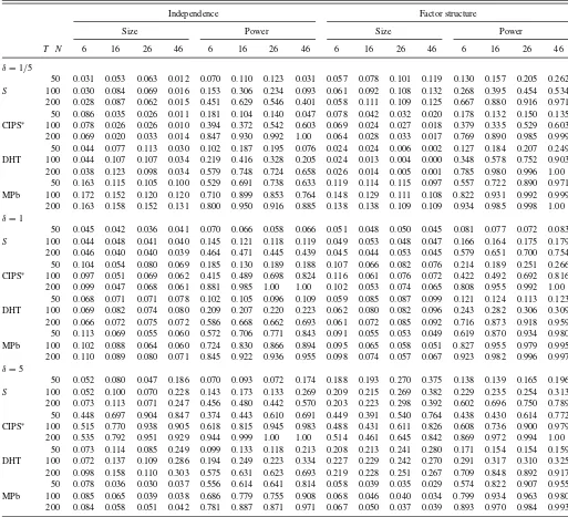
Table 1. Size and power of second-generation panel tests
Independence Factor structure
Size Power Size Power
T N 6 16 26 46 6 16 26 46 6 16 26 46 6 16 26 46
δ=1/5
50 0.031 0.053 0.063 0.012 0.070 0.110 0.123 0.031 0.057 0.078 0.101 0.119 0.130 0.157 0.205 0.262
S 100 0.030 0.084 0.069 0.016 0.153 0.306 0.234 0.093 0.061 0.092 0.108 0.132 0.268 0.395 0.454 0.534 200 0.028 0.087 0.062 0.015 0.451 0.629 0.546 0.401 0.058 0.111 0.109 0.125 0.667 0.880 0.916 0.971 50 0.086 0.035 0.026 0.011 0.181 0.104 0.140 0.047 0.078 0.042 0.032 0.020 0.178 0.132 0.150 0.135 CIPS∗ 100 0.078 0.026 0.026 0.010 0.394 0.372 0.542 0.603 0.069 0.024 0.027 0.018 0.379 0.335 0.529 0.603 200 0.069 0.020 0.033 0.014 0.847 0.930 0.992 1.00 0.064 0.028 0.033 0.017 0.769 0.890 0.985 0.999 50 0.044 0.077 0.113 0.030 0.102 0.187 0.195 0.076 0.024 0.024 0.006 0.002 0.127 0.184 0.207 0.249 DHT 100 0.044 0.107 0.107 0.034 0.219 0.416 0.328 0.205 0.024 0.013 0.004 0.000 0.348 0.578 0.752 0.903 200 0.038 0.123 0.098 0.034 0.579 0.748 0.724 0.658 0.026 0.014 0.005 0.001 0.785 0.980 0.996 1.00
50 0.163 0.115 0.105 0.100 0.529 0.691 0.738 0.633 0.119 0.114 0.115 0.097 0.557 0.722 0.890 0.971 MPb 100 0.172 0.152 0.120 0.120 0.710 0.899 0.853 0.764 0.148 0.129 0.111 0.108 0.822 0.931 0.992 0.999 200 0.163 0.158 0.152 0.131 0.800 0.950 0.916 0.885 0.138 0.138 0.109 0.109 0.934 0.985 0.998 1.00
δ=1
50 0.045 0.042 0.036 0.041 0.070 0.066 0.058 0.066 0.051 0.048 0.050 0.045 0.081 0.077 0.072 0.083
S 100 0.044 0.048 0.041 0.040 0.145 0.121 0.118 0.119 0.049 0.053 0.048 0.047 0.166 0.164 0.175 0.179 200 0.046 0.040 0.040 0.039 0.464 0.471 0.445 0.439 0.045 0.044 0.053 0.045 0.579 0.651 0.700 0.754 50 0.104 0.054 0.080 0.069 0.185 0.130 0.189 0.188 0.107 0.066 0.082 0.076 0.214 0.189 0.251 0.266 CIPS∗ 100 0.097 0.051 0.069 0.062 0.415 0.489 0.698 0.824 0.116 0.061 0.076 0.072 0.422 0.492 0.692 0.816 200 0.099 0.047 0.068 0.061 0.881 0.985 1.00 1.00 0.102 0.053 0.074 0.065 0.808 0.955 0.992 1.00
50 0.068 0.071 0.071 0.078 0.102 0.105 0.096 0.109 0.059 0.085 0.087 0.099 0.121 0.124 0.113 0.123 DHT 100 0.069 0.082 0.074 0.080 0.209 0.207 0.220 0.223 0.062 0.080 0.082 0.096 0.243 0.282 0.306 0.309 200 0.066 0.072 0.075 0.072 0.586 0.668 0.662 0.693 0.061 0.072 0.085 0.092 0.716 0.873 0.918 0.959 50 0.113 0.069 0.055 0.060 0.572 0.706 0.771 0.843 0.091 0.055 0.053 0.049 0.619 0.870 0.934 0.980 MPb 100 0.102 0.088 0.064 0.060 0.724 0.830 0.866 0.894 0.095 0.065 0.058 0.051 0.827 0.955 0.979 0.995 200 0.110 0.089 0.080 0.071 0.845 0.922 0.936 0.955 0.098 0.074 0.057 0.067 0.923 0.982 0.996 0.997
δ=5
50 0.052 0.080 0.047 0.186 0.070 0.093 0.072 0.174 0.188 0.193 0.270 0.375 0.138 0.139 0.165 0.196
S 100 0.052 0.100 0.070 0.228 0.143 0.173 0.133 0.269 0.209 0.215 0.269 0.382 0.229 0.235 0.254 0.313 200 0.073 0.113 0.071 0.247 0.456 0.480 0.442 0.570 0.203 0.223 0.298 0.392 0.602 0.696 0.750 0.789 50 0.448 0.697 0.904 0.847 0.374 0.443 0.610 0.691 0.449 0.391 0.540 0.764 0.438 0.430 0.614 0.772 CIPS∗ 100 0.515 0.770 0.938 0.905 0.618 0.815 0.945 0.983 0.488 0.431 0.611 0.826 0.608 0.736 0.900 0.979 200 0.535 0.792 0.951 0.929 0.944 0.999 1.00 1.00 0.514 0.461 0.645 0.842 0.869 0.972 0.994 1.00
50 0.073 0.114 0.085 0.249 0.099 0.133 0.118 0.213 0.208 0.213 0.241 0.280 0.171 0.154 0.154 0.159 DHT 100 0.072 0.137 0.109 0.286 0.194 0.249 0.223 0.334 0.227 0.229 0.242 0.270 0.291 0.317 0.310 0.325 200 0.098 0.158 0.110 0.303 0.575 0.631 0.623 0.693 0.219 0.228 0.251 0.267 0.709 0.848 0.892 0.917 50 0.078 0.036 0.030 0.037 0.556 0.614 0.641 0.814 0.058 0.039 0.035 0.029 0.574 0.822 0.907 0.955 MPb 100 0.085 0.065 0.039 0.038 0.686 0.779 0.755 0.908 0.068 0.046 0.040 0.034 0.799 0.934 0.963 0.980 200 0.084 0.058 0.051 0.042 0.781 0.887 0.871 0.971 0.067 0.050 0.037 0.039 0.893 0.970 0.984 0.993
NOTE: Nominal 5% level; 5000 replications;ζi∼U[0.1,0.9].Sis from Hanck (in press), CIPS∗is from Pesaran (2007), DHT is from Demetrescu et al. (2006), and MPb is from Moon and Perron (2004).
alternatives without short-run dynamics (ai,j =0), we obtain
µ=cµwithµ=E(01sgn(Wµ(s))W(s)ds). By simulation, we findµ≈0.461. Hence,τI Vhas higher local power than the test
of Im et al. (2003) [IPS], for which Harris, Harvey, Leybourne, and Sakkas (2010) found µ≈0.282 under a negligible ini-tial condition, the most favorable case for the Im et al. (2003) test.
4. SMALL-SAMPLE BEHAVIOR
Since we fit a constant throughout, we assume without loss of generality that E(yi,t)=0 in our DGP:
yi,t=ρiyi,t−1+εi,t i=1, . . . , N, t =1, . . . , T
The variance-breaking error processes are independent nor-mal variates ˜εi,t, where var(˜εi,t)=1 fort=1, . . . ,⌊ζiT⌋and
var(˜εi,t)=1/δ2 for t = ⌊ζiT⌋ +1, . . . , T. We consider δ∈
{1/5,1,5} and take ζi =ζ ∈ {0.1,0.5,0.9} or draw
hetero-geneous break dates randomly at ζi ∼U[0.1,0.9]. We
con-sider two patterns of cross-sectional correlation among the
εi,t: (a) Independence: εi,t=ε˜i,t, and (b) Factor Structure:
εi,t :=λi·νt+ε˜i,t, whereνtare iidN(0,1) andλi ∼U(−1,3).
When (φ1, . . . , φN)′=0N, we study the size of the tests. To an-alyze power, we draw theφi from the uniform distribution on
[−0.1,0].
Table 1reports results for some second-generation tests (i.e., tests robust to cross-sectional dependence, but that are not de-signed to handle nonstationary volatility) forζi ∼U[0.1,0.9].
Similar results for the other DGPs described above are available
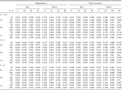
Table 2. Size and power of the Shin and Kang and Demetrescu et al. panel tests
Independence Factor structure
Size Power Size Power
T N 6 16 26 46 6 16 26 46 6 16 26 46 6 16 26 46
δ=1/5
50 0.054 0.049 0.039 0.044 0.175 0.244 0.235 0.159 0.043 0.042 0.038 0.029 0.268 0.400 0.454 0.387
τI V 100 0.053 0.059 0.055 0.045 0.359 0.526 0.510 0.456 0.047 0.040 0.040 0.034 0.608 0.840 0.951 0.984 200 0.049 0.058 0.052 0.052 0.593 0.852 0.840 0.843 0.048 0.047 0.049 0.040 0.922 0.996 1.00 1.00
50 0.047 0.047 0.047 0.041 0.172 0.228 0.236 0.170 0.037 0.038 0.032 0.035 0.195 0.287 0.347 0.342
PI V 100 0.049 0.057 0.051 0.043 0.392 0.534 0.600 0.648 0.042 0.037 0.039 0.032 0.496 0.746 0.891 0.953 200 0.049 0.052 0.053 0.048 0.701 0.900 0.935 0.971 0.045 0.042 0.043 0.041 0.882 0.992 1.00 1.00
50 0.049 0.059 0.054 0.041 0.105 0.106 0.099 0.113 0.040 0.035 0.029 0.023 0.133 0.135 0.135 0.110
tξˆ∗,κ 100 0.055 0.066 0.062 0.048 0.255 0.265 0.237 0.287 0.047 0.043 0.037 0.025 0.290 0.336 0.359 0.379 200 0.061 0.072 0.054 0.049 0.574 0.606 0.619 0.690 0.045 0.043 0.037 0.028 0.659 0.807 0.892 0.964
δ=1
50 0.046 0.046 0.045 0.048 0.177 0.219 0.243 0.214 0.041 0.034 0.035 0.027 0.268 0.417 0.489 0.439
τI V 100 0.048 0.050 0.048 0.051 0.363 0.483 0.566 0.664 0.046 0.043 0.036 0.034 0.566 0.850 0.932 0.978 200 0.048 0.047 0.050 0.054 0.636 0.830 0.905 0.969 0.051 0.052 0.044 0.042 0.897 0.992 0.999 1.00
50 0.041 0.038 0.041 0.043 0.169 0.225 0.248 0.219 0.034 0.031 0.031 0.030 0.211 0.324 0.393 0.396
PI V 100 0.043 0.044 0.044 0.042 0.395 0.581 0.672 0.758 0.042 0.039 0.037 0.032 0.498 0.790 0.906 0.966 200 0.049 0.048 0.047 0.046 0.754 0.942 0.979 0.998 0.047 0.046 0.040 0.039 0.883 0.992 1.00 1.00
50 0.046 0.038 0.038 0.035 0.120 0.111 0.110 0.109 0.042 0.049 0.045 0.041 0.142 0.126 0.124 0.098
tξˆ∗,κ 100 0.053 0.051 0.049 0.046 0.271 0.301 0.305 0.319 0.051 0.057 0.060 0.055 0.318 0.378 0.409 0.414 200 0.057 0.059 0.054 0.050 0.624 0.725 0.717 0.760 0.055 0.054 0.063 0.065 0.726 0.877 0.931 0.967
δ=5
50 0.045 0.041 0.039 0.040 0.173 0.176 0.157 0.192 0.040 0.033 0.029 0.029 0.192 0.315 0.362 0.311
τI V 100 0.049 0.045 0.048 0.041 0.338 0.353 0.369 0.553 0.048 0.037 0.038 0.032 0.411 0.678 0.784 0.852 200 0.048 0.049 0.049 0.043 0.507 0.630 0.716 0.883 0.046 0.046 0.043 0.041 0.714 0.949 0.985 0.996 50 0.038 0.032 0.030 0.038 0.197 0.246 0.247 0.198 0.034 0.028 0.028 0.028 0.154 0.258 0.315 0.283
PI V 100 0.047 0.037 0.035 0.039 0.444 0.567 0.676 0.656 0.040 0.032 0.030 0.029 0.384 0.673 0.795 0.876 200 0.047 0.044 0.040 0.038 0.697 0.877 0.964 0.962 0.044 0.043 0.039 0.036 0.734 0.971 0.995 1.00
50 0.046 0.037 0.034 0.021 0.106 0.096 0.114 0.071 0.046 0.046 0.042 0.047 0.108 0.101 0.091 0.087
tξˆ∗,κ 100 0.047 0.050 0.047 0.031 0.258 0.226 0.260 0.179 0.054 0.064 0.060 0.063 0.266 0.304 0.310 0.320 200 0.058 0.057 0.053 0.049 0.555 0.531 0.598 0.493 0.062 0.077 0.077 0.080 0.610 0.768 0.832 0.859
NOTE: Nominal 5% level; 5000 replications;ζi∼U[0.1,0.9].
upon request. All tests handle well the benchmark homoscedas-tic case δ=1. (For δ=1, the small-sample size distortions arise for instance because Pesaran (2007) tabulated critical val-ues starting with N =10, and we employ these for N =6.) The panels for the variance breaksδ=1/5 andδ=5 however clearly demonstrate that second-generation tests do not yield valid inference under nonstationary volatility.
We therefore turn our attention to robust tests. RegardingτI V,
the issue of interest is the behavior of the orthogonalization pro-cedure, so we simulate without short-run dynamics. We nev-ertheless include one lagged difference to capture the effect of not knowing the true lag order in practice. Hartung’s (1999) ap-proach to capture cross-sectional dependence assumes constant correlation. He proposed to estimate the off-diagonal element
ξ of the correlation matrix by ˆξ∗ =max((N−1)−1,ξˆ), where
ˆ
ξ =1−(N−1)−1N i=1(t
µ
I V ,i−N−1
N i=1t
µ
I V ,i)2 to form the
panel test statistic:
tˆξ∗,κ=
N i=1t
µ I V ,i
N+(N2−N)
ˆ
ξ∗+κ 2
N+1(1−ξˆ∗)
;
here, κ =0.1·(1+(N+1)−1
−ξˆ∗) improves the small-sample behavior oftˆξ∗,κ. The test rejects for large negative values
using standard normal critical values, see also Demetrescu et al. (2006).
Table 2reports rejection rates for Shin and Kang’s (2006)
τI V,PI V, andtξˆ∗,κ based on thet µ
I V ,i. Size is well-controlled
under both independence and cross-sectional dependence;τI V
is somewhat more accurate thanPI V ortˆξ∗,κ. As to power, all
tests are consistent asT → ∞for any configuration ofζandδ; power increases inN forT whenT is sufficiently large. Once more,τI V emerges as the most attractive choice: its power tends
to be higher than that of the other tests, although there are cases wherePI V is more powerful. Thetξˆ∗,κtest seems to have lower
power.
As pointed out above, the key drawback ofτI V is the
require-ment thatT > N for −1
ε to exist. This may not be the case
in practice. Moreover, ifT is only moderately larger than N, the finite-sample performance ofτI V will suffer. We therefore
employ a recent proposal by Ledoit and Wolf (2004) to estimate
ε allowing in principle any configuration ofT andN. They proposed to construct a weighted version ofεand the identity matrix I, ST =κ1TI+κ2Tε. Specifically, κ1T andκ2T are
Demetrescu and Hanck: Unit Root Testing in Heteroscedastic Panels 261
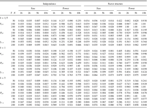
Table 3. Size and power of the Shin and Kang and Demetrescu et al. panel tests with shrinkage
Independence Factor structure
Size Power Size Power
T N 16 26 56 106 16 26 56 106 16 26 56 106 16 26 56 106
δ=1/5
50 0.024 0.035 0.007 0.020 0.144 0.217 0.090 0.253 0.034 0.036 0.023 0.014 0.422 0.682 0.820 0.930
τI V 100 0.033 0.041 0.019 0.032 0.419 0.588 0.472 0.813 0.039 0.040 0.036 0.024 0.888 0.987 1.00 1.00 200 0.039 0.048 0.038 0.044 0.746 0.913 0.882 0.998 0.043 0.047 0.038 0.028 0.999 1.00 1.00 1.00 50 0.006 0.006 0.000 0.000 0.057 0.058 0.002 0.001 0.015 0.013 0.001 0.000 0.201 0.367 0.301 0.195
PI V 100 0.014 0.013 0.001 0.000 0.431 0.458 0.441 0.328 0.018 0.022 0.005 0.000 0.730 0.929 0.979 0.996 200 0.029 0.028 0.014 0.006 0.873 0.946 0.977 0.997 0.030 0.031 0.011 0.003 0.995 1.00 1.00 1.00
50 0.045 0.049 0.040 0.048 0.106 0.099 0.114 0.092 0.032 0.028 0.020 0.020 0.143 0.134 0.092 0.050
tξˆ∗,κ 100 0.053 0.052 0.044 0.052 0.254 0.251 0.285 0.248 0.039 0.032 0.028 0.024 0.351 0.363 0.335 0.364 200 0.053 0.069 0.055 0.063 0.643 0.630 0.691 0.666 0.043 0.035 0.029 0.029 0.803 0.910 0.962 0.997
δ=1
50 0.034 0.030 0.016 0.005 0.190 0.215 0.198 0.137 0.029 0.024 0.009 0.001 0.405 0.484 0.551 0.463
τI V 100 0.039 0.037 0.034 0.026 0.488 0.562 0.672 0.731 0.041 0.032 0.027 0.014 0.843 0.933 0.986 0.996 200 0.041 0.048 0.048 0.046 0.817 0.892 0.973 0.995 0.044 0.044 0.041 0.039 0.993 0.999 1.00 1.00
50 0.013 0.007 0.000 0.000 0.124 0.115 0.032 0.000 0.013 0.008 0.000 0.000 0.238 0.259 0.138 0.002
PI V 100 0.025 0.020 0.010 0.001 0.536 0.623 0.658 0.459 0.031 0.022 0.011 0.001 0.760 0.877 0.959 0.950 200 0.034 0.036 0.029 0.018 0.929 0.974 0.997 1.00 0.038 0.036 0.032 0.019 0.996 0.999 1.00 1.00
50 0.043 0.039 0.034 0.027 0.106 0.108 0.107 0.103 0.040 0.042 0.044 0.034 0.131 0.109 0.082 0.059
tξˆ∗,κ 100 0.051 0.045 0.040 0.045 0.314 0.305 0.318 0.321 0.047 0.056 0.059 0.057 0.391 0.404 0.403 0.424 200 0.055 0.057 0.047 0.051 0.702 0.718 0.763 0.775 0.061 0.064 0.073 0.073 0.879 0.925 0.975 0.987
δ=5
50 0.014 0.017 0.009 0.001 0.134 0.168 0.193 0.092 0.025 0.020 0.005 0.001 0.275 0.319 0.344 0.261
τI V 100 0.026 0.026 0.028 0.007 0.359 0.442 0.595 0.588 0.033 0.032 0.019 0.009 0.627 0.743 0.890 0.929 200 0.040 0.041 0.034 0.022 0.614 0.784 0.931 0.957 0.038 0.037 0.032 0.025 0.933 0.980 0.998 1.00
50 0.003 0.002 0.000 0.000 0.073 0.054 0.017 0.000 0.010 0.004 0.000 0.000 0.146 0.131 0.038 0.000
PI V 100 0.010 0.006 0.003 0.000 0.469 0.446 0.432 0.269 0.022 0.015 0.004 0.000 0.578 0.704 0.808 0.676 200 0.023 0.019 0.013 0.001 0.833 0.908 0.970 0.979 0.029 0.027 0.019 0.006 0.955 0.991 1.00 1.00
50 0.042 0.028 0.019 0.035 0.100 0.086 0.053 0.106 0.048 0.048 0.047 0.039 0.098 0.097 0.077 0.077
tξˆ∗,κ 100 0.047 0.042 0.032 0.038 0.249 0.211 0.189 0.280 0.068 0.070 0.067 0.067 0.286 0.322 0.312 0.305 200 0.059 0.050 0.042 0.050 0.589 0.533 0.521 0.665 0.066 0.074 0.082 0.080 0.752 0.805 0.858 0.888
NOTE: Nominal 5% level; 5000 replications;ζi∼U[0.1,0.9].
constructed as follows. Define
¯
b2T = 1 N
⎡ ⎣
T
t=p+2
ε′
tεt
T
2
− 1
Ttr
2
ε
⎤ ⎦.
Further, mT =tr(ε)/N, dT2 =tr[(ε−mTI)(ε−
mTI)′]/N, bT2 =min( ¯b
2
T, d
2
T) and a
2
T =d
2
T −b
2
T. Then,
κ1T =mT ·b2T/d
2
T andκ2T =aT2/d
2
T. The full-rank matrix I
ensures that ST is invertible even if T < N. The (generally misspecified, but invertible) structure imposed by addingκ1TI
to the unbiased estimator ε introduces a finite-sample bias in ST. Yet, the weightsκ1T andκ2T are optimal in the sense
that ST asymptotically (forN, T → ∞jointly) has minimum expected loss in a class of linear combinations of I andε. Ledoit and Wolf (2004) showed the joint asymptotics to be a good guide in finite samples, including the case T < N. Moreover, the following lemma showsST to converge toat the same rate asεunder the assumptions of Proposition 2, so it can be safely used for the test of Shin and Kang (2006).
Lemma 2. Under the assumptions of Proposition 2, it holds that
ST − =Op(N T−0.5).
Proof. See the Appendix.
We now present additional simulations gauging the effective-ness of Shin and Kang’s (2006) tests using shrinkage, allowing us to also consider the case T < N. Table 3 reports rejection rates forN ∈ {16,26,56,106}. ThePI V test is now sometimes
drastically undersized especially forN≫T. Reassuringly, this does not destroy its consistency as PI V remains powerful at
least for largeT. On the other hand,τI V mostly performs quite
well even with shrinkage and in cases whereN > T, although predictably somewhat less accurately than when one can use an estimatorεthat unbiasedly estimates the true covariance ma-trix. In terms of size,tξˆ∗,κ, not requiring shrinkage, emerges as a
serious competitor whenN > T. However,τI V is substantially
more powerful thantˆξ∗,κfor small and intermediateTwhenever
size is comparable. Overall, these results lead us to recommend to employτI V in cross-dependent panels.
5. CONCLUDING REMARKS
The Cauchy estimator, for which the sign of the lagged level instruments the lagged level itself, yields a unit root test with an asymptotic standard normal null distribution even under uncon-ditional heteroscedasticity.
The article showed that the features of the Cauchy test ex-tend in cross-dependent, heteroscedastic panels. In particular, we prove the panel unit root test due to Shin and Kang (2006) to be robust to unconditional heteroscedasticity. Moreover, the test was shown to be locally more powerful than the IPS test of Im et al. (2003).
The assumptions under which jointN, T asymptotics hold suggested that Nshould be smaller thanT. To extend the ap-plicability of the panel test to situations whereTis comparable with, or smaller than,N, we proposed the use of shrinkage co-variance matrix estimators. The test performed well in small samples.
APPENDIX: PROOFS
Note: Sums run fromt=p+2 toTunless specified other-wise, andCstands for a generic constant.
Proof of Lemma 1. Note that it suffices to show that
T−1ε
i,tεj,t is
√
T-consistent at a uniform rate over 1≤
i, j ≤N (recall that the norm of anN×N matrix with uni-formly bounded elements isO(N)). To this end, we make use of the factor structure of the innovations. We namely have that
T−1εi,tεj,t =T−1
using the obvious uniform boundedness ofωiacross the panel,
we obtain that
irrespective ofi.The same reasoning applies to the other cross-products as well, leading with the summability conditions in As-sumption 3(b) to sup1≤i,j≤N var(T−
1ε
i,tεj,t −i,j)≤C/T.
Thus the sample covariances ofεtare√T-consistent for the re-spective elements of, as required.
Proof of Proposition 2. Let us first analyze the behavior of the sample covariance matrix ofεt,ε=T−1ε
tε′t. Note that
εi,t =εi,t+Op(T−0.5) (whether estimating by imposing the
unit root or not); we have at the assumed maximal rate forN
thatT−1(ε
tε′t−
ε
tε′t) =Op(N T−0.5); so, considering
Lemma 1, it follows that
ε−=Op(N T−0.5). (A.1)
Now making use of Equation (11b) from L¨utkepohl (1996, p. 107), we have that
Due to the factor structure of the innovations,has eigenval-ues bounded away from zero, hence−1< C; considering that ε−→p 0, the denominator of the right-hand side converges in probability to 1 and the numerator to zero at rate
Op(N T−0.5). This implies the same convergence rate of each
As in Lemma A.1B from Demetrescu and Hanck (2011) (DH), we have that E(|h2
duced using the same arguments as for the derivations below,
hi(xi,tµ−1)ε∗i,t=Op(
√
T), it follows from dividing denomi-nator and numerator byT1/2and using a Taylor expansion that
using arguments analogous to those used for Lemma A.1E in DH, we conclude that for all 1≤k, i≤N,
Demetrescu and Hanck: Unit Root Testing in Heteroscedastic Panels 263
So the elements of theN×N matrix T−1/2ε
th′t are
uni-formly bounded in probability, and
The norm on the left-hand side thus vanishes, implying that the trace vanishes too. Summing up, we have that
τI V =
Using again Lemma A.1E in DH as above, it follows im-mediately thatτI V =(T N)−1/2h′tŴ′εt+op(1); lettingıt = order moments (cf. Assumption 3), the second condition of the Central Limit Theorem (CLT) for md arrays (Davidson,1994, Thm. 24.3) is fulfilled. Checking the first condition amounts to showing that T−1(N−0.5ı′
Proof of Proposition 3. Begin by examining, like in the proof of Proposition 2, the quantity
1
We show that the trace vanishes under the local alternative as well. Withφi =(ρi−1)Ai, where theAihave been defined for
each unit after Assumption 1, we have that
T uniformlyL2-bounded, we have as in Lemma A.1E in DH that
cal alternative too, so the proof of Lemma 1 still applies leading toŴ−Ŵ =Op(N2T−0.5),and the trace does indeed vanish like in the proof of Proposition 2. Use now the Cauchy–Schwarz inequality and Lemma A.1B in DH together with the uniform
L2-boundedness ofxk,t−1/
LettingC =diag(ciAi) (the diagonal matrix with diagonal
el-ementsAici) and recalling thatŴ=diag(ω−i1),we have as in
the proof of Proposition 2 that
τI V =
examine the noncentrality term of τI V’s asymptotic
distribu-tion: use the independence of the units and the uniform L2
-boundedness (ini) ofT−1sgn(xµ decomposition and the uniform boundedness of the variances imply
A Taylor series expansion for rα with rest term in
dif-ferential form, rα
=r0α+α̺α−1(r
leading with Minkowski’s inequality and (A.2) to
To conclude about the convergence of the expectation of the left-hand side to the expectation on the right-hand side of (A.3), note that the sequence T−1.5sgn(xµ
i,t−1)xi,t−1 is uniformly L2-bounded (intas well as ini) and as such uniformly integrable. So convergence of the expectations holds, as required for the result.
Proof of Lemma 2. SinceST− ≤ ST−ε + ε− , we only have to prove that ST −ε =Op(N T−0.5)
thanks to (A.1). With I =1, ST −ε ≤ |κ1T| + |κ2T − 1|ε. Since ε =Op(N),|κ2T −1| =b2
T/d
2
T andmT =
1
Ntr(ε)=
1
N T N i=1ε
2
it =Op(1), proving ST −ε =
Op(N T−0.5) reduces to showing
bT2
dT2 =Op(T −0.5
).
An upper bound for b2T is derived as follows. Recall, b2T =
min( ¯b2T, dT2) with ¯b2T =((ε′
tεt/T)2−tr(
2
ε)/T)/N. Due to
the symmetry ofε,the trace on the right-hand side amounts to the sum of the squared elements of ε; the elements have uniformly bounded variance (cf. the proof of Lemma 1), so the squares have uniformly bounded expectation and thus T−1tr(2
ε)=Op(N2T−1). It then follows analogously
that (ε′
tεt/T)2=Op(N2/T2) and thus ¯bT2 =Op(N T−1). Since
bT2 =min( ¯b2T, dT2),we need a lower bound fordT2.The trace in-volved in the expression ofdT2 amounts to the sum of squared elements ofε−mTI.Due to the√T-consistency of the
ele-ments ofε,we have
dT2 =tr−mTI −mTI′/N+Op(N T−0.5).
TheOp term on the right-hand side indicates an upper bound,
though, so we derive the desired lower bound fordT2 from the behavior of −mTI. In fact it is sufficient to examine , given thatmT =Op(1). Under Assumption 3(a), tr(
2
) is of exact magnitude orderN2, so tr((−mTI)(−mTI)′)/N is bounded away from zero (it is in fact of order at leastN) and
b2
T =Op(N/T).Using again the fact thatdT2is of order at least
N,we obtain that
b2
T
d2
T
=Op
1
T
,
which is sufficient for the result.
ACKNOWLEDGMENT
The authors would like to thank an anonymous referee and an associate editor, as well as Peter Boswijk, J¨org Breitung,
Hashem Pesaran, and Werner Ploberger for very helpful com-ments and suggestions.
[Received January 2011. Revised October 2011.]
REFERENCES
Bai, J., and Ng, S. (2004), “A PANIC Attack on Unit Roots and Cointegration,”
Econometrica, 72, 1127–1177. [258]
Boswijk, H. P. (2005), ‘‘Adaptive Testing for a Unit Root With Nonstation-ary Volatility,” UvA-Econometrics Discussion Paper 07, Universiteit van Amsterdam. [258]
Breitung, J., and Das, S. (2005), “Panel Unit Root Tests Under Cross Sectional Dependence,”Statistica Neerlandica, 59, 414–433. [257]
Cavaliere, G. (2004), “Unit Root Tests Under Time-Varying Variances,” Econo-metric Reviews, 23, 259–292. [256]
Cavaliere, G., and Taylor, A. M. R. (2007), “Testing for Unit Roots in Time Series Models With Non-Stationary Volatility,”Journal of Econometrics, 140, 919–947. [257]
Davidson, J. (1994),Stochastic Limit Theory, Oxford: Oxford University Press. [263]
Demetrescu, M., and Hanck, C. (2011), “IV Estimators for Autoregressive Processes Under Nonstationary Error Volatility,” Technical Report, De-partment of Economics, Universit¨at Bonn. Available at http://www.ect.uni-bonn.de/mitarbeiter/prof.-dr.-matei-demetrescu/robust-iv-autoregression. [256,257,262]
Demetrescu, M., Hassler, U., and Tarcolea, A.-I. (2006), “Combining Signif-icance of Correlated Statistics With Application to Panel Data,”Oxford Bulletin of Economics and Statistics, 68, 647–663. [257]
Hanck, C. (in press), “An Intersection Test for Panel Unit Roots,”Econometric Reviews. [259]
Harris, D., Harvey, D. I., Leybourne, S. J., and Sakkas, N. D. (2010), “Local Asymptotic Power of the Im-Pesaran-Shin Panel Unit Root Test and the Impact Of Initial Observations,”Econometric Theory, 26, 311–324. [259] Hartung, J. (1999), “A Note on Combining Dependent Tests of Significance,”
Biometrical Journal, 41, 849–855. [256,258,260]
Im, K. S., Pesaran, M. H., and Shin, Y. (2003), “Testing for Unit Roots in Heterogeneous Panels,”Journal of Econometrics, 115, 53–74. [259,262] Ledoit, O., and Wolf, M. (2004), “A Well-Conditioned Estimator for
Large-Dimensional Covariance Matrices,”Journal of Multivariate Analysis, 88, 365–411. [260,261]
L¨utkepohl, H. (1996),Handbook of Matrices, New York: Wiley. [262] Moon, H. R., and Perron, B. (2004), “Testing for a Unit Root in Panels With
Dynamic Factors,”Journal of Econometrics, 122, 81–126. [257,259] Pesaran, M. H. (2007), “A Simple Panel Unit Root Test in the Presence of
Cross Section Dependence,”Journal of Applied Econometrics, 22, 265– 312. [257,259,260]
Shin, D. W., and Kang, S. (2006), “An Instrumental Variable Approach for Panel Unit Root Tests Under Cross-Sectional Dependence,”Journal of Economet-rics, 134, 215–234. [256,257,258,260,261]
Shin, D. W., and Lee, O. (2001), “Tests for Asymmetry in Possibly Nonstationary Time Series Data,”Journal of Business and Economic Statistics, 19, 233– 244. [256]
——— (2003), “An Instrumental Variable Approach for Tests of Unit Roots and Seasonal Unit Roots in Asymmetric Time Series Models,”Journal of Econometrics, 115, 29–52. [256]
So, B. S., and Shin, D. W. (1999), “Cauchy Estimators for Autoregressive Processes With Applications to Unit Root Tests and Confidence Intervals,”
Econometric Theory, 15, 165–176. [256,257]
Stock, J. H., and Watson, M. W. (2002), “Has the Business Cycle Changed and Why?,”NBER Macroeconomics Annual, 17, 159–218. [256]