Objective Bayesian Approach for SNP Data:
Method, Simulation Study and Application
Adi Setiawan
Program Studi Matematika, Fakultas Sains dan Matematika
Universitas Kristen Satya Wacana Jl. Diponegoro 52-60 Salatiga 50711 Indonesia ([email protected])
Abstract
Bayesian inference is often criticized for its reliance on prior distributions, whose choice influences the conclusion. In particular, in testing theory the necessity of assigning prior probabilities to the two hypotheses appears awkward. The objective Bayesian approach overcomes this criticism by an objective choice of priors. It aims at producing inference statements that only depend on the assumed model and the available data. In this paper we propose to use objective Bayesian approach to find genes associated to the complex disease of interest by using SNP (single nucleotide polymorphism) as a marker. Simulation study is then used to describe the properties of this approach. Finally this approach is used in the whole-genome SNP data of cases and controls sample in case-control association study.
Keywords: Objective Bayesian, single nucleotide polymorphism, case-control association study, intrinsic statistics.
Introduction
Genetic epidemiologists have taken the challenge to identify genetic polymorphisms involved in the development of complex diseases. Statistical methods have been developed for analyzing the relation between genetic polymorphisms such as SNP (single nucleotide polymorphism) to complex disease in genetic association studies (for example, see [6], [4] and [1]). In this paper, it is described an objective Bayesian approach for analyzing SNP data in case-control association studies. In case case-control studies, we compare the genotypes of individuals who have a disease (cases) with the genotype of individuals without the disease (controls). The proportions in each group having a characteristic of interest (for instance the number of genotypes of a given type) are then compared to determine whether there is an association between the complex disease and the characteristic of interest. The properties of objective Bayesian approach are described by using simulation. Finally this approach is used in the whole-genome SNP data.
Statistical Method
Suppose that we observe data X whose distribution is governed by a parameter θ belonging to a parameter set Θ and we wish to investigate whether
θ belongs to a subset Θ0⊂ Θ. Given a prior on Θ and a function δ( θ , Θ0) measuring discrepancy between a parameter θ and the null parameter set Θ0, it is natural to base inference on the posterior discrepancy
∫δ θΘ π θ θ
=
Θ X X d
d( 0, ) ( , 0) ( | ) ,
where π(θ | X) is the posterior distribution of θ. Bernardo and Rueda [2] propose to use a reference
prior and the (symmetrized) Kullback-Leibler divergence as the discrepancy measure. The latter is defined as
} ) ) | ( , ) | ( (
, )) | ( ), | ( ( min{ inf ) , (
0
0 0
0 0
θ θ
θ θ =
Θ θ δ
Θ ∈ θ
x p x p K
x p x p K
(1)
for x→p(x | θ ) the density of X and K the Kullback-Leibler divergence of p1 from p2
dx x p
x p x p p p
K ∫
⎟⎟⎠ ⎞ ⎜⎜⎝ ⎛ =
) (
) ( log ) ( ) , (
2 1 1
2
1 .
Bernardo and Rueda [2] call equation (1) based on these choices the intrinsic statistic. Reference priors are proposed as consensus priors designed to have a minimal effect, relative to the data, on the posterior inference. If the observed data X follows a smooth one-parameter model, the reference prior will be the Jeffreys' prior, i.e. π(θ) ∝ i(θ)1/2 and for a k -parameter model where k > 1, we can also use Jeffreys' prior, but then
[
]
21
) ) ( det( )
(θ∝ θ
π i ,
where i(θ) is the Fisher information function.
We shall apply this approach to testing whether the distributions of two independent observations X
and Y are governed by the same parameters. The full parameter is a pair ( θ,θ′) ranging over a product set and the observation (X,Y) possesses density
(x,y) →p(x|θ) p(y|θ′ ).
our examples these are the Jeffreys' priors. The intrinsic statistic can be considered a measure of evidence against the null model. Bernardo and Rueda [2] claim that the numerical value may be interpreted on an absolute scale independent of sample size and dimensionality. The null model is false if the intrinsic statistic d(Θ0,(X, Y)) is sufficiently large. Formally, if
d(Θ0,(X, Y)) ≤ 2.5 then we have no evidence that the null model is false, if 2.5 < d(Θ0,(X, Y)) ≤ 5 then we have mild evidence that the null model is false, if 5 < d(Θ0,(X, Y)) ≤ 8.5 then we have strong evidence that the null model is false, and finally if d(Θ0,(X, Y )) > 8.5 then we have conclusive evidence that the null model is false.
Single Marker Genotype-Based Method
The methods are based on a case-control design and try to find marker loci that are associated to the disease by comparing genotype frequencies between random samples of cases (diseased individuals) and controls. The methods can be classified as single marker, double marker or multiple markers according to whether they take into account frequencies of markers at one locus or combinations of markers at two or more loci. In current practice, phase is not observed, i.e. the raw data consists of unordered genotypes at the marker loci and not of multi-locus haplotypes. For single marker methods phase is not considered important, because it is commonly assumed that parental and maternal origins of alleles are not important for determining phenotype. Single marker methods are, however, classified as
allele-based or genotype-allele-based according to whether they assume Hardy-Weinberg equilibrium or not. If pAA,
pAa and paa are the relative frequencies of genotypes
AA, Aa, aa in the population, then Hardy-Weinberg equilibrium is said to hold if
pAA = pA 2, pAa = 2 pA pa, paa = pa2
for pA and pa = 1 - pA the frequencies of alleles A and
a in the population. Allele based single marker methods parameterize the genotype frequencies through the single parameter pA, using the preceding
identities, whereas genotype-based methods let the vector ( pAA, pAa, paa ) vary freely over the
two-dimensional unit simplex. Under assumptions of infinite population size, discrete generations, random mating, no selection, no migration, no mutation and equal initial genotype frequencies in the two sexes, Hardy-Weinberg equilibrium arises after one generation and thereafter the genotype frequencies in the population are constant from generation to generation.
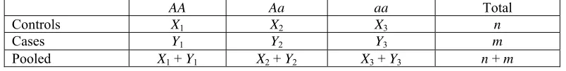
Let (p1, p2, p3) and (q1, q2, q3) be the genotype frequencies in the populations of controls and cases, respectively. We take random samples of n controls and m cases, respectively. The layout of the data is given in Table 1. Testing association between the genotype of the marker locus and the disease is equivalent to testing the null hypothesis H0 : p = q versus the alternative hypothesis H1 : p≠q where p = (p1, p2, p3) and q = (q1, q2, q3).
AA Aa aa Total
Controls X1 X2 X3 n
Cases Y1 Y2 Y3 m
Pooled X1 + Y1 X2 + Y2 X3 + Y3 n + m
Table 1. Table of the number of genotypes in control and case samples.
Suppose that random vectors X = ( X1, X2, X3 ) and Y = ( Y1, Y2, Y3 ) are the numbers of genotype AA,
Aa and aa in the samples of controls and cases, respectively. These vectors possess Multi(n, p) and Multi(m, q) distributions, respectively. The probability density function of X is
3 2 1
2 1 )
|
( px p x px
x n p x f
⎟⎟⎠ ⎞ ⎜⎜⎝ ⎛ =
where x1, x2, x3 = 0, 1, 2, ….. n, x1 + x2 + x3 = n, 0 <
p1, p2, p3 < 1, and p3 = 1 - p1 - p2 . The Fisher information matrix can be computed to be
⎟ ⎟ ⎟ ⎟
⎠ ⎞
⎜ ⎜ ⎜ ⎜
⎝ ⎛
− −− −
−
− − −
−− =
) 1
(
) 1 ( 1
1 1 )
1 (
) 1 (
) , (
2 1 2
1
2 1
2 1 2
1 1
2
2 1
p p p
p n p
p n
p p p
p p
p n
p p I
The reference prior is given by
1 2 1
3 1 2 1
2 1 2 1
1 2 1
3 2 1 1
1 )
( = − − −
⎟⎟⎠ ⎞ ⎜⎜⎝
⎛ ∝
π p p p
p p p p
Thus, the reference prior is the Dirichlet (
2
1
,
2
1
,
2
1
)-distribution. The reference prior for q is the same
distribution, and the reference prior for (p,q) is the independent combination of the two marginal priors. The joint probability density function of X and Y is
h(x,y | p, q) = f( x | p) g(y | q)
= 1 2 3 1 2 3.
3 2 1 3
2 1
y y y x
x x
q
q
q
y
m
p
p
p
x
n
⎟⎟⎠
⎞
⎜⎜⎝
⎛
⎟⎟⎠
Then the posterior density function of (p; q) given X
= x and Y = y is
[
]
⎟⎟⎠ ⎞ ⎜⎜⎝ ⎛ + ⎟⎟⎠ ⎞ ⎜⎜⎝ ⎛ + ⎟⎟⎠ ⎞ ⎜⎜⎝ ⎛ = 3 3 2 2 2 1 1 1 ) , ( log log log ] ) , ( | ) , ( [ r p X r p X r p X E s r q p K n q pπ3(p,q | x, y)
∝π1(p) π2(q) h(x, y | p,q)
∝ 3 2 1 3 2 1 3 2 1 3 2 1 1 2 1 3 1 2 1 2 1 2 1 1 1 2 1 3 1 2 1 2 1 2 1 1 y y y x x x
q
q
q
p
p
p
q
q
q
p
p
p
− − − − − −= 1 2 1 3 1 2 1 2 1 2 1 1 1 2 1 3 1 2 1 2 1 2 1 1 3 2 1 3 2 1 − + − + − + − + − + − + y y y x x x
q
q
q
p
p
p
.Thus the posterior π3(p,q | x, y) is the independent combination of the
Dirichlet ( y1 +
2
1
, y2 +
2
1
, y3 +
2
1
)
-distribution for p and the Dirichlet ( y1 +
2
1
, y2 +
2
1
, y3 +
2
1
)-distribution for q.
We wish to test the null hypothesis H0 : p = q. Let
Θ = { ( p, q) : 0 < p1, p2, p3 < 1, p1 + p2 + p3 = 1, 0 < q1, q2, q3 < 1, q1 + q2 + q3 = 1 }.
The quotient of the densities of (X;Y) for two parameter values (p; q) and (r; s) is given by
3 2 1 3 2 1 3 2 1 3 2 1 3 2 1 3 2 1 3 2 1 3 2 1 ) , | , ( ) , | , ( y y y x x x y y y x x x s s s r r r y m x n q q q p p p y m x n s r y x h q p y x h ⎟⎟⎠ ⎞ ⎜⎜⎝ ⎛ ⎟⎟⎠ ⎞ ⎜⎜⎝ ⎛ ⎟⎟⎠ ⎞ ⎜⎜⎝ ⎛ ⎟⎟⎠ ⎞ ⎜⎜⎝ ⎛ = 3 2 1 3 2 1 3 3 2 2 1 1 3 3 2 2 1 1 y y y x x x s q s q s q r p r p r p ⎟⎟⎠ ⎞ ⎜⎜⎝ ⎛ ⎟⎟⎠ ⎞ ⎜⎜⎝ ⎛ ⎟⎟⎠ ⎞ ⎜⎜⎝ ⎛ ⎟⎟⎠ ⎞ ⎜⎜⎝ ⎛ ⎟⎟⎠ ⎞ ⎜⎜⎝ ⎛ ⎟⎟⎠ ⎞ ⎜⎜⎝ ⎛ = and ⎟⎟⎠ ⎞ ⎜⎜⎝ ⎛ + ⎟⎟⎠ ⎞ ⎜⎜⎝ ⎛ + ⎟⎟⎠ ⎞ ⎜⎜⎝ ⎛ = ⎟⎟⎠ ⎞ ⎜⎜⎝ ⎛ 3 3 3 2 2 2 1 1 1 log log log ) , | , ( ) , | , ( log r p x r p x r p x s r y x h q p y x h
⎟⎟⎠
⎞
⎜⎜⎝
⎛
+
⎟⎟⎠
⎞
⎜⎜⎝
⎛
+
⎟⎟⎠
⎞
⎜⎜⎝
⎛
+
3 3 3 2 2 2 1 11
log
log
log
s
q
x
s
q
x
s
q
y
.The Kulback-Leibler divergence between the probability density functions h(x, y | p, q) and h(x, y |
r, s) is the expected value of this expression under parameter value (p, q)t, given by
+
[
]
⎟⎟⎠ ⎞ ⎜⎜⎝ ⎛ + ⎟⎟⎠ ⎞ ⎜⎜⎝ ⎛ + ⎟⎟⎠ ⎞ ⎜⎜⎝ ⎛ 3 3 3 2 2 2 1 1 1 ) ,( log log log
s q Y s q Y s q Y
E pq
⎟⎟⎠ ⎞ ⎜⎜⎝ ⎛ + ⎟⎟⎠ ⎞ ⎜⎜⎝ ⎛ + ⎟⎟⎠ ⎞ ⎜⎜⎝ ⎛ = 3 3 3 2 2 2 1 1
1log log log
r p p n r p p n r p p n + ⎟⎟⎠ ⎞ ⎜⎜⎝ ⎛ + ⎟⎟⎠ ⎞ ⎜⎜⎝ ⎛ + ⎟⎟⎠ ⎞ ⎜⎜⎝ ⎛ 3 3 3 2 2 2 1 1
1log log log
s q q m s q q m s q q m
= n L( p | r ) + mL( q | s ), where ⎟⎟⎠ ⎞ ⎜⎜⎝ ⎛ + ⎟⎟⎠ ⎞ ⎜⎜⎝ ⎛ + ⎟⎟⎠ ⎞ ⎜⎜⎝ ⎛ = 3 3 3 2 2 2 1 1
1log log log
) | ( r p p r p p r p p r p L .
The intrinsic discrepancy between h(x, y | p, q) and
h(x, y | p0, q0) where (p0, q0) ranges over Θ0 is
} ] ) , ( | ) , ( [ , ] ) , ( | ) , ( [ { min inf )] , ( , [ 0 0 0 0 0 0 q p q p K q p q p K q
p = p
θ δ
,
where the infimum is taken over all probability vectors p0 = (p01, p02, p03). Then the intrinsic statistic is given by
∫∫
Θ
=
Θ
p qdq
dp
y
x
q
p
q
p
q
p
d
)
,
|
,
(
]
)
,
(
,
[
]
)
,
(
,
[
0 0π
δ
.The intrinsic statistic cannot be found in closed form, but may easily be computed by Monte Carlo integration.
In the following, we illustrate the techniques on data collected by the Department of Medical Genetics at the Vrije Universiteit Medical Center Amsterdam. The genotype of data came from a genetically isolated population in Turkey with current population size around 6000 people. Ninety percent of these people are supposed to be descendants of 23 families that originally inhabited the region approximately 400 years ago. Genotyping was done using the Affimetrix 10K SNP chip to 27 controls and 31 cases We summarized characteristics of the 11229 SNPs, such as the identity of the SNP in the chromosome and the genotype of every individual in the control and case samples The genotype of individuals are defined as
AA, AB or BB, a missing genotype is coded as “NoCall”, meaning that the marker did not pass the discrimination filter [7].
conclusive evidence that there is an association between the marker and the disease.
AA Aa aa Total
Controls 11 14 2 27
Cases 29 2 0 31
Pooled 40 16 2 58
Table 2. Table of the number of genotypes in control and case samples.
Simulation Study and Application
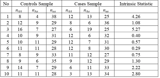
Genotype AA, Aa and aa are generated for 50 individuals in controls sample by using parameter (pAA, pAa,paa) = (0.2, 0.2, 0.6). Simulated data for 50
individuals in cases sample can be generated in a similar way. The result of simulated data in controls sample, cases sample and the related intrinsic statistic are given in Table 3. Based on the table, we conclude that the intrinsic statistic tends to give no evidence that the model is false (there is no association between the marker and the disease). Table 4 presents simulated data and their intrinsic statistic when we use parameter (pAA, pAa,paa) = (0.2, 0.2, 0.6) and (0.2,
0.6, 0.2) to generate controls sample and cases sample, respectively. Based on the table, as we expect, the intrinsic statistic tends to give strong
evidence that the model is false (there is an association between the marker and the disease).
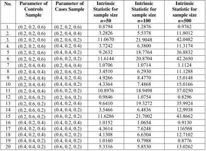
Simulation can be extended to different sample size. Table 5 presents the result of intrinsic statistic by using sample size 50, 100 and 500. We conclude that the greater sample size will have the greater intrinsic statistic.
[image:4.595.163.420.93.146.2]Objective Bayesian approach can then be applied to each SNP in the whole-genome 10K SNP data. In this approach, a SNP is called associated to the complex disease of interest if the intrinsic statistic is larger than 5. As the method claims to produce a measure of evidence that can be interpreted on an absolute scale, no correction for multiple testing appears to be necessary. Based on this approach, we find 111 associated markers.
Table 3. The result of simulated data in 50 controls sample, 50 cases sample and the related intrinsic statistic.
No Controls Sample Cases Sample Intrinsic Statistic nAA nAa naa nAA nAa naa
1 8 4 38 12 13 25 4.26
2 12 9 29 8 6 36 1.08
3 16 7 27 6 19 25 5.27
4 10 9 31 12 6 32 0.40
5 10 11 29 12 7 31 0.57
6 11 11 28 12 8 30 0.29
7 8 9 33 11 12 27 0.75
8 9 6 35 9 12 29 1.30
9 14 7 29 6 11 33 2.22
10 11 11 28 3 13 34 2.80
Table 4. The result of simulated data in 50 controls sample, 50 cases sample and the related intrinsic statistic.
No Control Sample Cases Sample Intrinsic Statistic nAA nAa naa nAA nAa naa
1 9 9 32 7 29 14 9.28
2 10 11 29 13 30 7 11.99
3 8 14 28 5 31 14 6.02
4 9 11 30 13 27 10 9.07
5 12 7 31 13 23 14 7.81
6 17 7 26 13 26 11 9.22
7 11 12 27 11 33 6 12.32
8 8 12 30 8 29 13 7.09
[image:4.595.138.467.409.571.2]10 4 13 33 15 27 8 14.08
Table 5. Relation between parameter, intrinsic statistic and sample size that is used to generate controls sample and cases sample.
No. Parameter of Controls
Sample
Parameter of Cases Sample
Intrinsic Statistic for sample size
n=50
Intrinsic Statistic for
sample size n=100
Intrinsic Statistic for sample size
n=500
1. (0.2, 0.2, 0.6) (0.2, 0.2, 0.6) 0.8794 1.2876 0.9762 2. (0.2, 0.2, 0.6) (0.2, 0.4, 0.4) 3.2826 5.5378 11.8012 3. (0.2, 0.2, 0.6) (0.2, 0.6, 0.2) 11.0670 21.9048 42.0482
4. (0.2, 0.2, 0.6) (0.4, 0.2, 0.4) 3.7242 6.3800 11.3174 5 (0.2, 0.2, 0.6) (0.4, 0.4, 0.2) 9.2632 18.7764 36.8832 6 (0.2, 0.2, 0.6) (0.6, 0.2, 0.2) 11.6144 20.8704 42.2650
7 (0.2, 0.4, 0.4) (0.2, 0.4, 0.4) 1.0706 1.0714 1.1124 8 (0.2, 0.4, 0.4) (0.2, 0.6, 0.2) 3.4510 6.2930 11.1288 9 (0.2, 0.4, 0.4) (0.4, 0.2, 0.4) 4.9266 8.4770 15.0148
10 (0.2, 0.4, 0.4) (0.4, 0.4, 0.2) 4.3364 7.4868 15.0166 11 (0.2, 0.4, 0.4) (0.6, 0.2, 0.2) 10.8976 18.9498 37.0250
12 (0.2, 0.6, 0.2) (0.2, 0.6, 0.2) 0.9846 1.0754 0.8296 13 (0.2, 0.6, 0.2) (0.4, 0.2, 0.4) 9.6410 19.3272 35.9924
14 (0.2, 0.6, 0.2) (0.4, 0.4, 0.2) 3.5466 6.4836 12.9938 15 (0.2, 0.6, 0.2) (0.6, 0.2, 0.2) 11.6286 21.7002 43.8662 16 (0.4, 0.2, 0.4) (0.4, 0.2, 0.4) 1.0152 1.0654 0.9130 17 (0.4, 0.2, 0.4) (0.4, 0.4, 0.2) 4.3614 7.6248 116568 18 (0.4, 0.2, 0.4) (0.6, 0.2, 0.2) 4.1308 6.6304 12.7102 19 (0.4, 0.4, 0.2) (0.4, 0.4, 0.2) 1.0160 0.7988 0.8776 20 (0.4, 0.4, 0.2) (0.6, 0.2, 0.2) 5.3316 5.8530 13.0262
Discussion
In this paper, we have explained an objective Bayesian approach to analyze SNP data in case-control association studies. A simulation study is done to describe the properties of objective Bayesian approach and then it is applied in the whole-genome association studies. The research can be extended for SNP data that use more than 200 K SNPs in whole-genome as in paper [5].
References
[1] Balding, D. J. 2006. A tutorial on statistical methods for population association studies. Nature Reviews Genetics 7 : 781.
[2] Bernardo, J. M. & Rueda, R. 2002. Bayesian Hypothesis Testing : A Reference Approach, International Statistical Review 70, 351-372. [3] Bernardo, J.M., (2005) Reference Analysis,
Handbook of Statistics 25, Amsterdam : Elsevier, 17-90.
[4] Heidema, A. G., J. M.A. Boer, N. Nagelkerke, E. C. M. Mariman, D. L. Van der A, E. J. M. Feskens. 2006. The challenge for genetic epidemiologist : how to analyze large numbers
of SNPs in relation to complex diseases, BMC Genet. 7:23
[5] Hoggart, C. J, J. C. Whittaker, Maria De Iorio, D. J. Balding. 2008. Simultaneous Analysis of All SNPs in Genome-Wide dan Re-Sequencing Association Studies, Plos Genetics, Volume 4 Issue 7.
[6] Hu, N., C. Wang, Y. Hu, H. H. Yang, C. Giffen, Z. Tang, X. Han, A. M. Goldstein, M. R. Emmer-Buck, K. H. Buetow, P. R. Taylor, M. P. Lee. 2005. Genome-Wide Association Study in Esophageal cancer Using GeneChip mapping 10K Array. Cancer Research 65 (7) : 2542-2546.