HYBRID GA-SQP ALGORITHMS FOR
THREE-DIMENSIONAL BOUNDARY DETECTION PROBLEMS IN POTENTIAL CORROSION DAMAGE
Nicolae S Mera
Abstract. In this paper we consider the identification of the geometric structure of the boundary of the solution domain for the three-dimensional Laplace equation. Cauchy data consisting of boundary measurements of cur-rents and voltages on the remainder of the boundary are used to determine the material loss caused by corrosion. This problem arrise in the early de-tection of corrosion in aging aircraft components. The domain identification problem is considered as a variational problem to minimize a defect functional, which utilises some additional data on certain known parts of the boundary. A sequential quadratic programming (SQP) optimisation algorithm and a real coded genetic algorithm (GA) are combined in order to obtain a fast algorithm that can deal with the multimodal objective function. The unknown boundary is parameterized using B-splines. The Laplace equation is discretised using the method of fundamental solutions (MFS). Numerical results are presented and discussed for four hybrid algorithms and several test examples.
2000 Mathematics Subject Classification: 65N21, 68T20, 90C56. 1. INTRODUCTION
action to remove and arrest corrosion of structure. As the age of an aircraft increases, the importance of detection of corrosion increases because there is an increased probability of an interaction between the corrosion and other forms of damage such as fatigue cracks. The detection of corrosion without disassembly of the aircraft prevents the possibility of aggravating the issue by removing effective sealant.
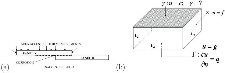
The most common technique for detection corrosion in aircraft is visual in-spection for surface distortions or pillowing of the outer skin. However, special non destructive techniques must be applied when regions are partially or com-pletely inaccessible for inspection due to the overlying structure. In airplanes, corrosion may occur in relatively inaccessible locations, such as within the lap joints of the skin of an airplane as is shown schematically in Figure 1(a). Two aluminum panels A and B overlap and corrosion may occur at the joint. One side of the aircraft skin is not accessible for inspection, so any damage on this side has to be identified from measurements available on the accessible side.
An electric voltage is applied to the aircraft skin, on the upper part and
(a)
PANEL A
PANEL B
INACCESSIBLE AREA AREA ACCESSIBLE FOR MEASUREMENTS
CORROSION
(b)
Figure 1: (a) Schematic drawing of two overlapping panels in an aircraft skin with corrosion occurring at the joint and (b) Problem formulation: the domain and the boundary conditions of the 3D problem considered.
[image:2.595.107.476.334.454.2]In this paper the problem of boundary detection is reformulated as an optimisation problem and the unknown boundary is sought in a B-splines parametric form. Thus the problem is regularized by using the function spec-ification method, i.e. by assuming a parametric form of the unknown function and reducing the problem to the determination of a reduced number of pa-rameters, i.e. the control points of the B-splines surface. We note that once the problem has been formulated as an optimisation problem then various optimisation algorithms may be used in order to locate the optimum of the objective function. The efficiency of a particular optimisation method clearly depends on the form of the objective function. In the problem considered in this paper, the objective function has a complex nonlinear and nonmonotonic structure. Both heuristic methods such as genetic algorithms (GAs) see Mera et al. [7] and deterministic methods such as sequential quadratic programming (SQP), see Mera and Lesnic [8] have been successfully applied to optimise this function. Evolutionary algorithms search the whole space being able to deal with multi-modal functions and discontinuities. Deterministic, gradient based optimisation methods do not search the full parameter space and can tend to converge toward local extrema of the fitness function, which is clearly un-satisfactory for problems where the fitness varies nonmonotonically with the parameters. On the other hand in vicinity of local optima the rates of con-vergence exhibited by the gradient based algorithms clearly outperform those of evolutionary algorithms, see Mera et al. [9]. Therefore it is the purpose of this paper to formulate hybrid algorithms that incorporate the advantages of both deterministic and heuristic optimisation algorithms.
2. MATHEMATICAL FORMULATION
In this paper the EIT is used to determine material loss occurring on the inaccessible portion γ ⊂ ∂Ω of the boundary ∂Ω of a domain Ω ⊂ R3 by
measuring voltages and currents (Cauchy data) on an accessible portion of the boundary. Therefore, we consider the Laplace equation in a three-dimensional damaged finite plate Ω for the potential u, namely,
subject to the boundary conditions u =g, ∂u
∂n =q on Γ (2)
α0u+β0
∂u
∂n =f on Σ (3)
α1u+β1
∂u
∂n =h on γ (4)
wheref, g, h, q, α0, β0, α1 and β1 are prescribed functions andn is the outward
normal to the boundary ∂Ω. In eqns (2)−(4) the boundaries γ,Γ and Σ are disjoint and γ ∪Γ∪Σ = ∂Ω. The problem investigated consists of determin-ing the shape of the unknown boundary γ given the boundary data specified by eqns (2)−(4). This problems occurs in several contexts, such as corrosion detection by electrostatic measurements, see Kaup and Santosa [5]. Several computational results for the two-dimensional case can be found in the lit-erature, using, for example, Tikhonov regularization in connection with the L-curve method, see Kaup et al. [6]. Charton et al.[1] proposed a variational technique based on parameterising the unknown boundary using the function specification method. For the three dimensional case a sequential quadratic programming method of solution was developed in Mera and Lesnic [8] while the same problem was investigated using a genetic algorithm in Mera et al [7].
3. THE METHOD OF SOLUTION
3.1 Reformulation as an optimisation problem
The boundary detection problem given by eqns (1)-(4) can be reformulated as an optimisation problem. For a given possible solution γ for the unknown boundary, the following direct problem is solved:
∇2u= 0, in Ω (5)
u=g, on Γ (6)
α0u+β0
∂u
∂n =f on Σ (7)
α1u+β1
∂u
and the current flux on the known boundary u′
calc = ∂u∂n
Γ is evaluated. The
solution of the problem may be found by minimising the functional J(γ) =ku′
calc−qkL2(Γ) (9)
where q is the measured current flux on the boundary Γ. The boundary γ can be parameterised in different forms and the parameters characterising the shape of the boundary are determined by minimising the functional (9). In this paper we have used B-splines to parameterise the unknown surface γ. 3.2 The parametrisation of the boundary by B-splines surfaces The unknown boundary γ is sought in the parametric form
γ(v, w) =
n X i=0 m X j=0
Ni,k(v)Nj,l(w)Pij, (v, w)∈[0,1]×[0,1] (10)
whereNi,k andNj,l are thekth and lth degree B-spline basis functions given by
Ni,0(v) = χ[vi,vi+1]; Ni,k(v) =
v −vi
vi+k−vi
Ni,k−1+
vi+k+1−v
vi+k+1−vi+1
Ni+1,k−1 (11)
Nj,0(w) =χ[wj,wj+1]; Nj,l(w) =
w−wj
wj+l−wj
Nj,l−1+
wj+l+1−w
wj+l+1−wj+1
Nj+1,l−1
(12) defined on the nonperiodic, nonuniform knot vectors V = (vi)i=0,n+k+1 and
W = (wi)i=0,m+l+1, see Piegl and Tiller [13]. The points Pij are the control
points of the B-spline surfaceγand they determine the shape of this boundary. Thus, the problem of boundary detection is reduced to determining the (m+ 1)(n+ 1) control points Pij. The x and y coordinates of the control points
are considered to be known while the z coordinate is to be detected. In the problem considered in this paper we assume that the intersection between the boundary γ and Σ is known, i.e. we know the curves that form the boundary of the surfaceγbut we don’t know it’s internal shape. Thus, the control points Pij with i∈ {0, n}or j ∈ {0, m} are known and the only unknowns are thez
coordinates of the remaining control points. Thus, the problem of boundary identification is reduced to determining the components of the matrix
Z zPij
i=1,n−1,j=1,m−1 =
zP11 zP12 ... zP1,m−2 zP1,m−1
... ... ... ... ... zPn−1,1 zPn−1,2 ... zPn−1,m−2 zPn−1,m−1
It should be noted that the ill-posed problem of identifying the boundary of the domain is regularized by using the function specification method, i.e. by assuming a pre-defined shape and reducing the problem to the determination of the parameters of the B-spline surface. In the more general case when no parametric shape is assumed for the boundaryγ then the problem is ill-posed and regularization terms must be included in the objective functional (9). By using such regularization terms that penalize non-smooth solutions, and choos-ing the appropriate regularization parameter, a stable numerical solution can be obtained.
3.3 The method of fundamental solutions
A meshless method, namely the method of fundamental solution, see Fair-weather and Karageorghis [2], is used to solve the direct problem (5)-(8) and to evaluate the objective function (9) for a given boundary γ. The numerical solution is developed by using the fundamental solution of the Laplace equa-tion as a basis funcequa-tion.
In order to introduce the method of fundamental solutions, we consider the entire domain Ω and we consider a set of M nodal pointsxi, i= 1, M outside
Ω. The fundamental solution of the three-dimensional Laplace eqn.(5) is given by:
F(x) = 1
4πkxk (14)
Then the fundamental solutions centered at the nodal pointsxi,i= 1, M given by
φi(x) =F(x−xi) =
1
4πkx−xik (15)
satisfy the partial differential eqn.(5). The method of fundamental solutions is based on the fact that an approximation to the solution of the direct problem (5)-(8) can be expanded in terms of these basis functions, φi, i.e. the solution
is sought in the form:
u∗(x) = M X
i=1
αiφi(x) (16)
where αi are unknown coefficients. For this choice of basis functions the
ap-proximated solutionu∗already satisfies the Laplace eqn.(5) and the coefficients
αi, i = 1, M, are determined such that u∗ satisfies the boundary conditions
We consider N collocation points xj, j = 1, N on the boundary of the domain Ω. Using the given values of the voltage (or current flux) at these N collocation points, then the resulting system of linear algebraic equations for the unknown coefficients αi is obtained by collocating (16) at the points xj,
j = 1, N and a system of linear algebraic equations,
Aα=b (17)
is obtained, where the vectorαcontains the unknown coefficientsαi,i= 1, M.
It should be noted that in order to uniquely determine the coefficients αi,
i = 1, M the number of collocation points N must be greater or equal to the number of nodal points M.
However, the system of linear algebraic equations is ill-conditioned and can-not be solved by direct methods, such as the least squares methods, since such an approach would produce a highly unstable solution. Most standard numer-ical methods cannot achieve good accuracy in solving the matrix eqn.(17) due to the large value of the condition number of the matrixAwhich increases dra-matically with respect to increasing the total number of collocation points and nodal points. Several regularization methods have been developed for solving these kind of ill-conditioned problems, see Hansen [4]. In this study we use the standard Tikhonov regularization method, see Tikhonov et al. [21].
The Tikhonov regularized solutionαλfor eqn.(17) is defined as the solution of the following least squares problem:
min
α {kAα−bk+λ
2kαk} (18)
where k · k denotes the usual Euclidean norm and λ is the regularization pa-rameter.
The choice of a suitable value of the the regularization parameter λ is crucial for the accuracy of the final numerical solution and there are several methods for determining an optimal value for this parameter, such as the L-curve method, Hansen [3], the discrepancy principle, Tikhonovet al. [14], etc. In this study we use the L-curve method, i.e. we define the curve
point of maximum curvature of the L-curve, see Hansen [3].
For the problem of boundary detection, the MFS is particularly suitable since the geometry of the system changes for every possible solution tested during the optimisation process. Further, MFS does not require any mesh-ing of the domain or the boundary in order to calculate the boundary data. This reduces the computational effort and eliminates the important pertur-bations due to changes in the mesh. MFS also is known to be very efficient from the point of view of the computational time required to solve a linear direct problem such as (5)-(8). The MFS can be also used to compute values very near to, or even on the boundaries, and there is no singularity in the solution, as the nodal points are always placed outside the solution domain. The MFS is also suitable for high-dimensional problems and irregular domains. 3.4 Optimisation algorithms
The boundary identification problem (1)-(4) has been solved in Mera et al. [9] by using two different algorithms, one deterministic, gradient based optimisa-tion algorithm and one heuristic, evoluoptimisa-tionary search algorithm. We consider again the same algorithms, namely, as a gradient based optimisation algorithm we use the sequential quadratic programming optimisation algorithm E04UCF from the NAG Libraries, see NAG [12] and for the evolutionary search we con-sider a float number encoded genetic algorithm proposed in Meraet al. [7] with population size npop = 10, number of offspringnchild = 15, uniform arithmetic
crossover, crossover probability pc = 0.65, tournament selection, tournament
size k = 2, tournament probability pt = 0.8, non-uniform mutation, mutation
probability pm = 0.5, elitism, elitism parameter ne = 2. The float number
encoding of the variables enables natural implementation of fine local tuning processes. Indeed the non-uniform mutation operator is an operator that en-ables fine local tuning and causes the GA to search the space uniformly initially and locally at later stages.
gradi-ent methods may fail to locate the global optimum. It should be noted that similar results have been obtained for the two-dimensional case. It was found in Charton et al. [1] that the numerical solutions obtained by the Gradient Projection Method (GPM) or Nelder-Mead Simplex Method (NMNS) depend on the initial guess specified. For some initial guesses, these gradient based methods converge toward local optima which are far from the real solution for the boundaryγ. On the other hand, the genetic algorithm, starting with a ran-dom initial population, was always found to converge to the global optimum. In general, it in known that genetic algorithms have the ability to escape lo-cal optima and therefore they are particularly suitable for nonlinear functions with complex, highly structured landscape which can appear in shape optimi-sation problems. One disadvantage of genetic algorithms, in comparison with gradient methods, is the increased amount of computational time required for the evolutionary search process.
In order to combine the advantages of the two optimisation methods we consider the following four hybrid algorithms.
H1 - Several GA generations are performed in order to identify the most promising areas and then the SQP optimisation algorithm is applied using as an initial guess the best individual found by the GA. It should be noted that in this approach the GA is used to specify a good initial guess for the SQP algorithm.
H2 - A SQP operator is introduced in the GA scheme. The effect of this operator is equivalent to executing 5 SQP steps on the selected individ-ual. In the H2 algorithm during every generation the SQP operator is applied to the best individual in the population, i.e. every generation 5 SQP steps are executed starting from the best individual and the result is introduced back in the GA population.
H3 - The same SQP operator as in H2 algorithm is used but it is applied to all members of the GA population, once every 10 generations.
These four hybrid algorithm are tested on several test examples in order to identify their performance and limitations.
4. NUMERICAL RESULTS
In order to test the convergence and the stability of the methods proposed, we use as the solution domain the thin plate illustrated in Figure 1(b). The lengths of the domain are taken to be Lx =Ly = 1.0 and Lz = 0.1 althought
it was found that stable computations can be performed up to Lz = 0.5, see
Mera and Lesnic [8]. The unknown boundaryγ is assumed to be maintained at constant voltage, sayu=c, while a Dirichelet boundary condition is prescribed on Σ and Cauchy boundary conditions are prescribed on Γ. The method of fundamental solution, see section 3.3, is used to solve the direct problem (5)-(8) and to evaluate the objective function (9) for a given boundary γ. In all the results presented in this paper, N = 150 collocation points have been uniformly distributed on the boundary ∂Ω and M = 150 nodal point have been distributed on the boundary of a cube of side length L = 3.0 that includes in the interior the solution domain Ω. In this section we consider the retrieval of the boundaryγ given by various shapes parameterized by B-splines as described in section 3.2. For the numerical test examples considered in this paper we use cubic B-splines, i.e. k = l = 3 and we set m =n = 4, i.e. the surface γ is given by (m+ 1)(n+ 1) = 25 control points. The knot vectors are taken to be
U =V = (0,0,0,0,1
2,1,1,1,1) (20)
The x and y coordinates of the control points are given by xPi,j =−
Lx
2 + i
nLx, i= 0, n, j = 0, m (21) yPi,j =−
Ly
2 + j
mLy, i= 0, n, j = 0, m (22) The z coordinates of the control points Pij with i ∈ {0, n} or j ∈ {0, m} are
fixed toz = 0.5Lz, sinceγ T
various sequences of random numbers and the result presented is the average of the five runs.
The first test example considered is a unimodal, symmetrical test example given by eqn.(10) with
Z=
2.5Lz 2.5Lz 2.5Lz
2.5Lz 2.5Lz 2.5Lz
2.5Lz 2.5Lz 2.5Lz
(23)
and the search ranges for the z coordinates of the control points were set to be zmin = 0.1Lz and zmax = 3.0Lz.
In general, when using iterative methods, for solving ill-posed problems then a stopping criterion is required in order to regularize the problem. The iterative processes are not convergent with respect to the number of iterations due to the accumulation of noise effects. The real errors obtained by comparing the numerical solution with the exact solution decrease up to a specific point and then start increasing slowly, as the numerical solution loses its smoothness. Therefore regularizing stopping criteria are used in order to locate the optimum point in iterative methods for ill-posed problems. However, since we are using the function specification method, i.e. the solution is parametrized by B-splines, see section 3.2, the problem is regularized by looking for a solution in a parametric form depending on a reduced number of parameters. Therefore when only the parameters in eqn.(23) are to be retrieved, the iterative process is convergent with respect to the number of generations and simpler stopping criteria can be used, for example, one may stop the iterative process using a Cauchy type criterion, i.e. stop the iterative process when the solution does not change over a large number of iterations/generations.
(a)
0 200 400 600 800 1000 1200 1400
Number of evaluations 0.01
0.1 1.0 10.0 *10-1
Objective function
(b)
0 200 400 600 800 1000 1200 1400
Number of evaluations 1.0*10-4
1.0*10-3
1.0*10-2
1.0*10-1
[image:12.595.113.477.92.231.2]1.0*100
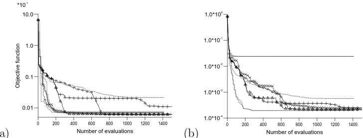
Figure 2: The evolution of the objective function as a function of the number of evaluations as obtained by various algorithm, namely H1 (◦), H2 (×), H3 (+), H4 (∆), GA (- - -) and SQP (· · · · ·) for (a) the test example given by equation 23 and (b) the test example given by equation 24
H3 the SQP operator is applied to every individual in the GA population and thus a large number of evaluations are wasted within SQP operators starting from neighboring initial guesses and from initial guesses which are not in the promising areas of the search space.
A non-symmetrical test example may be obtained by a B-spline surface given by eqn.(10) and the control points
Z=
2.5Lz 0.5Lz 0.5Lz
2.5Lz 0.5Lz 0.5Lz
2.5Lz 0.5Lz 0.5Lz
(24)
Two more complex boundary γ are considered by utilising the following
(a)
0 200 400 600 800 1000 1200 1400
Number of evaluations 0.01 0.05 0.1 0.5 1.0 5.0 10.0 *10-1 Objective function (b)
0 200 400 600 800 1000 1200 1400
Number of evaluations 1.0*10-4
1.0*10-3
1.0*10-2
1.0*10-1
[image:13.595.110.485.120.256.2]1.0*100
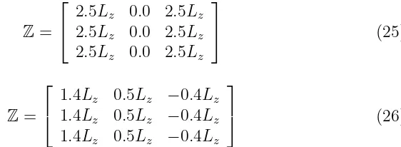
Figure 3: The evolution of the objective function as a function of the number of evaluations as obtained by various algorithm, namely H1 (◦), H2 (×), H3 (+), H4 (∆), GA (- - -) and SQP (· · · · ·) for (a) the test example given by equation 25 and (b) the test example given by equation 26
control points
Z=
2.5Lz 0.0 2.5Lz
2.5Lz 0.0 2.5Lz
2.5Lz 0.0 2.5Lz (25) and Z=
1.4Lz 0.5Lz −0.4Lz
1.4Lz 0.5Lz −0.4Lz
1.4Lz 0.5Lz −0.4Lz
(26)
[image:13.595.209.490.351.454.2]with the rate of convergence of the algorithm, and therefore the H2 algorithm may exhibit a poorer performance when compared to other hybrid algorithms. In the H3 algorithm by applying the SQP operator to all the individuals in the population, the dominance of only one individual is avoided. However, by applying SQP to all the individuals, a large number or evaluations are used for poor initial guesses and the rate of convergence of the algorithm is decreased. The H1 algorithm was found to be fast and accurate for all the test
[image:14.595.110.479.210.374.2](a) (b)
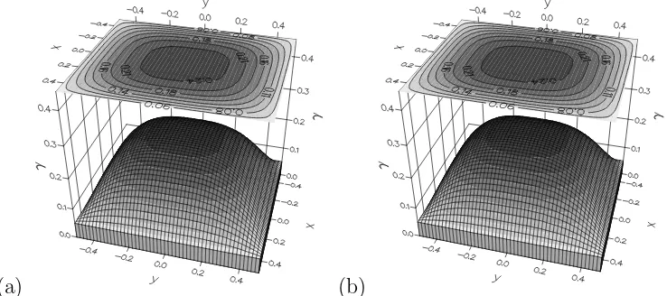
Figure 4: The exact (a) and the numerical (b) solution obtained by the H4 algorithm for the unknown boundaryγ for the test example given by equation (23) for s= 1% noise after 1000 evaluations.
examples. However, also this algorithm presents a drawback in the fact that the number of generations to be performed by the GA before switching to SQP optimisation cannot be determined a priori. There are no estimates of how many evaluations are required in order to drive the GA within the radius of convergence of the SQP. If too many generations are performed or if the GA is allowed to converge, the hybrid algorithm will have a global rate of convergence not faster that that of a standard GA. On the other hand, if the GA if not run for long enough, and it has not entered the zone of convergence of the SQP, then the hybrid algorithm does not benefit on the global search propoerties of the GA and it will possible converge to a local optima.
(a) (b)
Figure 5: The exact (a) and the numerical (b) solution obtained by the H4 algorithm for the unknown boundaryγ for the test example given by equation (24) for s= 1% noise after 1000 evaluations.
(a) (b)
Figure 6: The exact (a) and the numerical (b) solution obtained by the H4 algorithm for the unknown boundaryγ for the test example given by equation (25) for s= 1% noise after 1000 evaluations.
[image:15.595.105.480.334.499.2](a) (b)
Figure 7: The exact (a) and the numerical (b) solution obtained by the H4 algorithm for the unknown boundaryγ for the test example given by equation (26) for s= 1% noise after 1000 evaluations.
H1 algorithm. At the same time, the premature convergence which appears sometimes in the H2 algorithm is avoided by not introducing the SQP evolved individual back in the GA population. Thus, the GA is allowed to evolve and its global search properties are exploited without being affected by individuals with very good objective function generated by the SQP algorithm. In all the test examples investigated the H4 algorithm was found to converge to the real solution at a rate of convergence close to that of the SQP algorithm.
The numerical solutions obtained by the H4 using 1000 function evaluations for the four test examples considered are presented in Figures 4-7 in comparison with the exact solution. It can be seen that for all the test examples considered the numerical solution is a good approximations to the exact solution. Thus it can be concluded that using hybrid algorithms, complex boundaries can be retrieved within a small number of objective function evaluation.
5. CONCLUSIONS
optimisation techniques have been employed in order to find the optimal so-lution and hybrid SQP and GA methods have been compared on various test examples. It has been found that by combining GAs and SQP optimisation algorithms it is possible to generate hybrid algorithms that preserve the global search properties of the GA and at the same time exhibit local rates of conver-gence much faster that that of the standard GA and close to the SQP rate of convergence. Overall, the hybrid GQ-SQP algorithms were found to be fast, robust and accurate methods for boundary identification.
References
1. M. Charton, H.J. Reinhardt and D.N. Hao, Numerical solution of a shape optimisation problem, Eurotherm seminar 68, Inverse Problems and Ex-perimental Design in Thermal and Mechanical Engineering, Poitier, France, 2001, 101-105.
2. G. Fairweather and A. Karageorghis, The method of fundamental so-lutions for elliptic boundary value problems, Adv. Comput. Math., 9, 1998, 69-95.
3. P.C. Hansen, Analysis of discrete ill-posed problems by means of the L-curve, SIAM Review, 34, 1992, 561-580.
4. P.C. Hansen, Rank Deficient and Discrete Ill-Posed Problems: Numerical Aspects of Linear Inversion, SIAM, Philadelphia, 1998.
5. P.G. Kaup and F. Santosa , Nondestructive evaluation of corrosion dam-age using electrostatic boundary measurements, J. Nondestruct. Eval., 14, 1995, 127-136.
6. P.G. Kaup, F. Santosa and M. Vogelius, Method for imaging corrosion damage in thin plates from electrostatic data, Inverse Problems ,12, 1996, 279-293.
8. N.S. Mera and D. Lesnic, A three-dimensional boundary determination problem in potential corrosion damage, Comput. Mech., 36,2, 2005, 129-138.
9. N.S. Mera, L. Elliott, D.B. Ingham and D. Lesnic, A three-dimensional boundary determination problem in potential corrosion damage, 5th In-ternational Conference on Inverse Problems in Engineering, Theory and Practice, vol2, Leeds University Press, Leeds, M04, 2005.
10. Z. Michalewicz, Genetic Algorithms + Data Structures = Evolution Pro-grams, Springer-Verlag, Berlin, 1996.
11. V.A. Morozov, On the solution of functional equations by the method of regularization, Math. Dokl., 7, 1966, 414-417.
12. NAG Fortran Library Manual, Mark 18, The Numerical Algorithms Ltd., Oxford, 1999.
13. L. Piegl and W. Tiller, The NURBS book , Springer, Berlin, 1997. 14. A.N. Tikhonov, A.V. Goncharky, V.V. Stepanov and A.G. Yagola,
Nu-merical Methods for the Solution of Ill-Posed Problems, Kluwer Acad. Publ., Dordrecht, 1995.
Nicolae S Mera
Centre for Computational Fluid Dynamics University of Leeds
Leeds, LS2 9JT, UK