Dynamical Critical Exponent for Two-Species
Totally Asymmetric Dif fusion on a Ring
⋆Birgit WEHEFRITZ-KAUFMANN
Department of Mathematics and Physics, Purdue University, 150 N. University Street, West Lafayette, IN 47906, USA
E-mail: [email protected]
URL: http://www.math.purdue.edu/∼ebkaufma/
Received September 28, 2009, in final form April 30, 2010; Published online May 12, 2010 doi:10.3842/SIGMA.2010.039
Abstract. We present a study of the two species totally asymmetric diffusion model using
the Bethe ansatz. The Hamiltonian has Uq(SU(3)) symmetry. We derive the nested Bethe ansatz equations and obtain the dynamical critical exponent from the finite-size scaling properties of the eigenvalue with the smallest real part. The dynamical critical exponent is 3
2 which is the exponent corresponding to KPZ growth in the single species asymmetric
diffusion model.
Key words: asymmetric diffusion; nestedUq(SU(3)) Bethe ansatz; dynamical critical expo-nent
2010 Mathematics Subject Classification: 82C27; 82B20
1
Introduction
The single species asymmetric diffusion process has attracted and continues to attract a lot of interest. It is a driven diffusive system describing a stochastic movement of hard-core particles in one dimension, where movements to the left and right take place with different probabilities. There are many interesting applications to shock formation [1, 2, 3], traffic flow [4], biopoly-mers [5,6, 7] and other driven diffusive systems1. Since the underlying quantum spin chain is integrable, the powerful method of Bethe ansatz is applicable and was widely used in the past to obtain analytical results (see e.g. [8, 9, 10, 11, 12]). The two-species asymmetric diffusion problem however has been less investigated. While the stationary state has been studied in some detail [13,14,15,16,17], much less is known about the full dynamics of the system.
Some results for the dynamical phase diagram were obtained from the matrix product ansatz [18] (however these are restricted to certain regions of the full parameter space) and from numerical studies of the model [19].
Recently, the multi-species asymmetric diffusion model with open boundaries has sparked interest [20,21,22]. This case can also be tackled using the matrix product ansatz.
In [23] the dynamics of a particular choice of the model is studied where two species hop in opposite directions on a ring, the diffusion constant being different from the passing rate of particles of different species [24]. This model corresponds directly to two coupled Burgers equations or to a Burgers equation coupled to a diffusion equation. The dynamical scaling properties are calculated from the time-evolution of the two-point correlation functions, based
⋆This paper is a contribution to the Proceedings of the XVIIIth International Colloquium on Integrable
Sys-tems and Quantum Symmetries (June 18–20, 2009, Prague, Czech Republic). The full collection is available at
http://www.emis.de/journals/SIGMA/ISQS2009.html
on a numerical study. The dynamical critical exponent is consistent with a subtle double Kardar– Parisi–Zhang type scaling (in the sense of factorization).
An analytical study of the dynamical scaling of the multi-species asymmetric exclusion pro-cess was described by [25] who found a dynamical critical exponent of 32 from a Bethe ansatz calculation if the diffusion was asymmetric and a critical exponent of 2 for symmetric diffusion. In the present paper, we investigate the dynamical critical exponent for thetotally asymmetric diffusion process with equal rates which is a related but dynamically different model that will be precisely defined in Section2. We will derive the Bethe ansatz equations starting from theR -matrix of the totally asymmetric diffusion model, calculate the energy gap and from a finite-size scaling analysis extract the critical exponent.
1.1 Discussion of the literature about the two-species asymmetric dif fusion model
We will briefly survey the literature on the two-species asymmetric diffusion model. Although there seem to be several approaches building on previous work [25, 26, 27, 28] by trying to extract an appropriate limit to totally asymmetric diffusion, the details of each such strategy are not obvious, however, and one runs into serious difficulties and subtleties as we will explain. We found that instead of trying to tweak the calculations in an ad-hoc manner, it is clearer and simpler to start from scratch and derive the Bethe ansatz equations directly for the totally asymmetric case. With hindsight, our calculation provides a firm ground for future comparison which might also facilitate to formulate the correct limiting procedure.
The Bethe ansatz equations for the two-species asymmetric diffusion model were put forth in an article by Dahmen [26]. They depend on a parameter γ that is related to the asymmetric hopping rates by exp(γ) = q = qΓL
ΓR, where ΓL and ΓR describe the hopping rate to the left and right, respectively. It is not at all clear how to take the limit of one of these hopping rates going to zero directly in the Bethe ansatz equations. Since in the limitq→0 all the ratios tend to one, and even the usual rescaling of the roots by a factor of q does not work – the resulting equations either diverge or become trivial.
In the paper by Popkov at al. [27] Bethe ansatz equations for three-species models with different hopping rates for all six possible particles exchanges are derived from the matrix product ansatz. One of the cases they discuss is a particular asymmetric exclusion process where the hopping rates are coupled as gB0=gA0+gAB wheregB0,gA0 and gAB correspond to
the processesA+ 0→0 +A,B+ 0→0 +B and A+B →B+A, respectively (and the three other rates are set to zero). In this paper we will choose all three non-zero rates to be the same, so the model considered here is different.
Although the way Cantini [28] derives the Bethe ansatz equations for the case of asymmetric diffusion seems to be the most amenable for taking the limit to our model, however, he has introduced phase factors eν10,eν20,eν12 that remain in the Bethe ansatz equations, and it is not
clear which value they should take for the case of totally asymmetric diffusion.
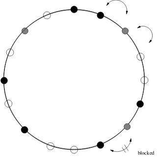
blocked
Figure 1. Example of totally asymmetric diffusion on a ring. Black dots correspond toAparticles, grey
dots toB particles and open dots to vacancies.
2
Two-species totally asymmetric dif fusion
2.1 Asymmetric dif fusion
The two-species asymmetric diffusion model consists of two species of particles, A and B, diffusing asymmetrically in one dimension. The following processes take place:
A+ 0→0 +A with rate ΓR, 0 +A→A+ 0 with rate ΓL,
B+ 0→0 +B with rate ΓR, 0 +B →B+ 0 with rate ΓL,
A+B →B+A with rate ΓR, B+A→A+B with rate ΓL.
2.2 Totally asymmetric dif fusion
In the totally asymmetric case, ΓL = 0, so particles A do not diffuse to the left since the
interchange B+A→A+B is blocked. This leads to a different dynamics for the model that will be analyzed in this article.
Assuming periodic boundary conditions, i.e. on the ring Z/LZ (where L is the number of
discrete sites of that ring), the model is shown qualitatively in Fig. 1. Diffusion to the right corresponds to clockwise motion around the circle, diffusion to the left to counterclockwise motion. Black dots represent particles A, grey dots particles B and open dots vacancies. The arrows indicate processes that are still allowed of ΓL= 0, the blocked arrow indicates the process
B+A→A+B that is forbidden in the totally asymmetric case.
ParticlesAdo not see any difference between vacant sites and particlesB, whereas particlesB
trying to diffuse to the right are blocked by particles A. Therefore, we call particles A “first-class”, and particles B “second-class” particles. There is an interesting connection between second-class particles and the study of current fluctuations [29].
2.3 Master equation and Hamiltonian
The dynamics of the asymmetric diffusion model is described by a master equation for the pro-bability distributionpt(η) of the lattice configurationη(t) at timet. If we denote a configuration
by η and the jump rates ΓR and ΓL by c(j, j+ 1, η), when interchanging the particles and/or
vacancies of the configurationη on sitesj and j+ 1, the master equation reads:
d
dtpt(η) = X
j
where ηjj+1 denotes the configuration obtained from η by interchanging the particles and/or vacancies at sites j and j+ 1. Following [30, 31], attaching a vector space C3 at each discrete
point j and using a vector (1,0,0)T for a particle of typeA, a vector (0,1,0)T for a particle of type B and a vector (0,0,1)T for a vacancy, the operator of the master equation can be written as a quantum spin chain which is given by the following expression if one assumes periodic boundary conditions
In the following, the standard vector space R3 will just be called V. In this expression, the
matrices Ejαβ are 3×3 matrices with only one non-zero entry: (Ejαβ)γδ=δαγδβδ and, as usual,
the expressionLP−1
j=1
EjαβEjβα+1 means theL-fold tensor product
111⊗112⊗ · · · ⊗11j−1⊗Ejαβ⊗Ejβα+1⊗11j+2⊗ · · · ⊗11L.
The parametersDandqare real and depend on the diffusion rates: q =qΓR
ΓL andD=
√
ΓRΓL.
This Hamiltonian is integrable and the eigenvalues can be found by applying the Bethe ansatz. Since the Hamiltonian is non-Hermitian in general, we will encounter complex eigenvalues.
2.4 Dynamical critical exponent
In non-equilibrium dynamics, the dynamical critical exponent describes a relation between the relaxation time towards equilibrium τ (or temporal correlation length) of a system and the spatial correlation lengthξ, namely that τ ≃ξz with the dynamical critical exponent z. It can be shown that for one-dimensional quantum spin chains, τ ≃ Lz. Since the relaxation time is
dominated by the eigenvalue of the Hamiltonian with the smallest real part (the energy of the ground state being equal to zero), we can obtain the exponent z from a finite size analysis of the Hamiltonian of the system as
Re (E1) = const
1
Lz. (2)
.
For the single species asymmetric diffusion model, z= 32 was obtained in [11] from a Bethe ansatz calculation for the totally asymmetric case which therefore belongs to the KPZ [32] universality class, whereasz= 2 for the partially asymmetric case which describes the Edwards– Wilkinson universality class [33]. We will determine the exponent zfrom a careful study of (2). We will find the lowest lying eigenvalue of the totally asymmetric diffusion model by means of the Bethe ansatz.
2.5 Nested Bethe ansatz
We start with the totally asymmetric diffusion model, setting the parameters ΓL = 0 and
ΓR= 1. This does not lead to any singularities in the Hamiltonian since its expression contains
This Hamiltonian is integrable, and we will use the algebraic Bethe ansatz to find its spec-trum. Although the Bethe ansatz is well known for the Hamiltonian (1), the totally asymmetric case (given by the Hamiltonian (3)) cannot be obtained as a special case since setting ΓL = 0
causes the Bethe ansatz equations to become singular. Therefore, we will derive the Bethe ansatz equations for the totally asymmetric case following [34,35]. We use the followingR-matrix ele-ments
Rαααα= expθ forα= 1, . . . ,3,
Rαββα= 2 sinhθ forα < β, α, β= 1. . . ,3, Rαββα= 0 forα > β, α, β= 1, . . . ,3, Rαβαβ = expθ forα < β, α, β = 1, . . . ,3, Rαβαβ = exp(−θ) forα > β, α, β = 1, . . . ,3,
where the indices denote the following tensor product in End(V ⊗V):
Rmkil Emi⊗Ekl,
or in the language of the associated vertex model this corresponds to the initial state denoted by the two indices miscattering into the final state denoted by the indices kl.
ThisR-matrix satisfies the factorization equation
Rjkpq(θ2−θ3)Riplr(θ1−θ3)Rrqmn(θ1−θ2) =Rqrij(θ1−θ2)Rrkpn(θ1−Θ3)Rpqlm(θ2−θ3).
We now define the 3L×3L matrices T(θ)[abL]as
T[L](θ)ab =
3 X
a1,...,aL−1=1
taa1(θ)⊗ta1a2(θ)⊗ · · · ⊗taL−1b(θ),
where
[tab(θ)]ij =Ribaj(θ), a, b, i, j = 1,2,3,
are 3×3 matrices. We define the monodromy matrix as
T[L]=
T11[L] T21[L] T31[L] T12[L] T22[L] T32[L] T13[L] T23[L] T33[L]
=
A B1 B2 C1 D11 D12 C2 D21 D22
. (4)
The monodromy matrix satisfies the fundamental relation
R(θ−θ′)[T[L](θ)⊗T[L](θ′)] = [T[L](θ′)⊗T[L](θ)]R(θ−θ′). (5) The transfer matrix
τ(θ) =
3 X
i=1 Tii(θ)
is obtained as the trace of the monodromy matrix. It is a matrix acting on V⊗L. In the above notation, it can be written as
τ(θ) =A(θ) +D11(θ) +D22(θ).
We recover the Hamiltonian (3) as the logarithmic derivative of the transfer matrix, if the spectral parameter θ is set to zero:
H = d(logτ(θ))
dθ
θ=0. (6)
2.6 Diagonalization of the transfer matrix
We start be deriving algebraic relations for the matrices A,Bj,Cj,j= 1,2 and Dik,i, k = 1,2
in equation (4).
Since we would like to diagonalizeτ, we are looking for a reference state that is a simultaneous eigenstate ofA and Dii and is annihilated by Ci and Dij fori6=j.
to be our reference state. This is not necessarily the physical ground state. T[L] acting on this reference state is interpreted as follows:
T[L]|Ωi=
acting on the reference state. They will be called creation operators in the following.
In the next step we use the fundamental relation equation (5) to derive the bilinear algebra among the operators A(θ), Bi(θ),Ci(θ) and Dij(θ).
The relations we are going to use later on are:
A(θ)Bi(θ′) =g(θ′−θ)Bi(θ′)A(θ)−h(θ′−θ)Bi(θ)A(θ′),
Bi(θ)Bj(θ) =rpqijBp(θ′)Bq(θ),
Dij(θ)Bk(θ′) =g(θ−θ′)rpqikBp(θ′)Djq(θ)−g(θ−θ′)Bi(θ)Djk(θ′). (9)
Hererpqij are coefficients of a 4×4 matrix where only the following five entries are different from
zero: r11
Now we are ready to look for an eigenstate of the transfer matrixτ(θ).
We will make the following ansatz for an eigenfunction of the transfer matrix having the creation operatorsBi(θ), i= 1,2 act on the reference state Ω given by equation (7).
We will calculate the action of the transfer matrix τ on the vector Ψ. Recall that τ =
A(θ) +D11(θ) +D22(θ). So we will encounter terms of the form
A(θ)Bσ(y1)(λ1)Bσ(y2)(λ2)· · ·Bσ(yp)(λp)|Ωi and
Dii(θ)Bσ(y1)(λ1)Bσ(y2)(λ2)· · ·Bσ(yp)(λp)|Ωi.
We know how A(θ) and Dii(θ) commute with the operators Bi(λj) from the relations (9) and
We will get two types of terms. In the first type of terms, we get the original combination of Bσ(y1)(λ1)Bσ(y2)(λ2)· · ·Bσ(yp)(λp)|Ωi back. They originate from taking the first term in the commutation relation for Bi(θ)Bj(θ) in (9). Using standard terminology, we will call those
termswanted terms. In the second type of terms, one of theBσ(yi) operators will depend on the parameter θ. These terms will be calledunwanted termsand their sum has to be set to zero.
We will also use the following notation: We define a 2p dimensional vector Bcontaining all
possible terms of the form Bσ(y1)(λ1)Bσ(y2)(λ2)· · ·Bσ(yp) where, as above, σ denotes a permu-tation of the set of indices {y1, y2, . . . , yp} ∈ {1,2}. We also define a 2p dimensional vector X
containing the correspondingxσ in the same order. This allows us to rewrite the sum as a scalar
product of these two vectors:
X
{σ}
xσBσ(y1)(λ1)Bσ(y2)(λ2)· · ·Bσ(yp)(λp) =B(λ1)⊗B(λ2)⊗ · · · ⊗B(λp)·X=B·X.
Then the action of the transfer matrix τ(θ) on Ψ(λ1, λ2, . . . , λp) leads to wanted terms that
can be written as:
a(θ)L
p
Y
i=1
g(λi−θ)Ψ(λ1, λ2, . . . , λp).
The unwanted terms arise from taking the second term in the commutation relation for the
B(θ) operators (9). E.g. one of the unwanted terms appears if the second term in the commutator is applied to A(θ)B(λk) and is of the form
h(λk−θ)a(λk)L p
Y
n6=k
g(λn−λk).
As observed by de Vega [36] the general unwanted term can easily written down if one uses the following fact about a cyclic permutation of poperators B(λj):
B(λ1)⊗B(λ2)⊗ · · · ⊗B(λp) =B(λ2)⊗B(λ3)⊗ · · · ⊗B(λp)⊗B(λ1)τ(2)p (λ1,{λ}),
where τ(2)p (θ,{λ}) = P2
a=1
Taa[p](θ,{λ}) and
Tab[p](θ,{λ}) =
2 X
a1,...,ap−1=1
t[2]aa1(θ−λ1)⊗t[2]a1a2(θ−λ2)⊗ · · · ⊗t [2]
ap−1b
(θ−λp),
where [t[2]ab(θ)]ij, a, b, i, j = 1,2 are 2×2 matrices where only the following five entries are
non-zero:
[t[2]11(θ)]11=r1111(θ), [t[2]11(θ)]22=r1221(θ), [t[2]21(θ)]21=r2121(θ),
[t[2]12(θ)]12=r1212(θ), [t [2]
22(θ)]22=r2222(θ).
Here rajib(θ) are the coefficients appearing in equation (9) andτ(2)p (θ,{λ}) is the transfer matrix of the six-vertex model (i.e. a model with two states instead of three states) for a line of psites with inhomogeneities {λi},i= 1, . . . , p.
So the cyclic permutationB(λi)→B(λi+1) followed by the multiplication of the matrix
leaves the productB(λ1)⊗B(λ2)⊗ · · · ⊗B(λp) invariant. Therefore the general unwanted term
Using the same argument as before, the general unwanted term can be written as a sum of terms where B(θ) replaces B(λk):
Altogether, the sum of wanted terms reads
B(λ1)⊗B(λ2)· · · ⊗B(λp)[a(θ)L
The sum of unwanted terms reads:
−
Since we are looking for an eigenstate of the transfer matrix, the sum of all wanted terms has to be proportional to |Ψi and the sum of all unwanted terms has to be equal to zero. The first condition determinesXto be an eigenvector ofτ(2)(p)corresponding to the eigenvalue Λ(2)(θ,{λ}):
τ(2)(p)X = Λ(2)(θ,{λ})X. (10)
The eigenvalue Λ(2)(θ,{λ}) is determined by requiring the sum of unwanted terms to become zero:
we have to do now is repeat the same diagonalization procedure for equation (10). We repeat exactly the same steps as before, acting with the transfer matrix on a reference state with r
creation matrices B, and deriving equations for the wanted and unwanted terms.
This leads to another expression for the eigenvalueλ(2)that can be set equal to equation (11) and another consistency equation stemming from setting the unwanted terms equal to zero. In this way we obtain the following nested Bethe ansatz equations which have two types of unknowns,λk,k= 1, . . . , pand Λj,j = 1, . . . , r,
The eigenvalues of H are obtained using the relation between the transfer matrix and the Hamiltonian given by equation (6):
E = d
2.7 Numerical solution of the Bethe ansatz equations
Since the Hamiltonian (3) is describing a reaction-diffusion system, the ground state is the steady state with energy zero and all excitation energies will have positive real parts. We fixedL,p andr and solved the coupled system of Bethe ansatz equations numerically. We also diagonalized the Hamiltonian (3) numerically for a small number of sites (typically up toL= 9). We compared the energies obtained from the Bethe ansatz with the ones obtained by numerical diagonalization of Hamiltonian H to single out the eigenvalue with the smallest non-zero real part which plays the role of the second lowest eigenvalue and determines the gap. This first excited state always lies in the sector with p = L3, r = 0. This state has an equal density of particles A, B and vacancies of 13. We extrapolated the energy values of the first excited state forL→ ∞.
2.8 Results
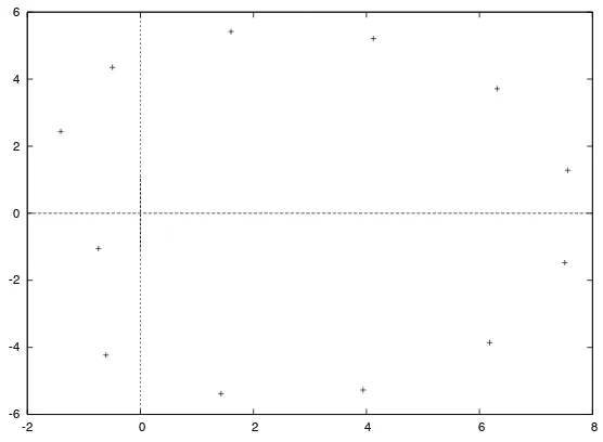
We found the solution for p= L3,r = 0 corresponding to the first excited state of Hamiltonian. To make sure that this really is the lowest lying excited state, we compared to the results of a numerical diagonalization of the Hamiltonian for finite lattice lengths. This state has an equal density of particles A, B and vacancies of 13. The roots all lie in the complex plane. A typical pattern of roots for the first excited state of the Hamiltonian is shown forL= 36 in Fig.2. The solid line is the unit circle that is given as a guide to the eye.
The data was extrapolated using the Bulirsch–Stoer algorithm [37]. Since we expect a scaling of the form (remember the ground state energy is always zero)
Re (∆E(L)) = Re (E1(L)) = constL−z+o(L−z),
we built extrapolants for the exponent−z as
LogRe (∆Re (∆EE(L(L+3))))
LogLL+3
-1
The data used in the extrapolation for the exponent is shown in table:
L extrapolant 6 −1.6336892192762 9 −1.6252314332778 12 −1.6092183117219 15 −1.5952666540982 18 −1.5839870664789 21 −1.5749003909369 24 −1.5674968193872 27 −1.5613778750522 30 −1.5562495252464 33 −1.5518961566109
The result of the extrapolation with BST-algorithm is−z=−1.50000009 with error 0.00000323. This clearly shows that the exponent z is 32.
It is interesting to note that this state corresponds to the Bethe ansatz equations with only one type of roots. The vanishing of the second type of roots does not correspond to the simple inclusion of the one-species model into the two-species model given by making the density of the second type of particles zero but rather for the state we consider corresponds to equal densities of these in-equivalent particles. The fact that the densities are coupled may suggest that there is some underlying quasi-particle formalism which may give a theoretical way to explain the connection to the single species exclusion model and the occurrence of the exponent 32 well known from the totally asymmetric single species exclusion model.
2.9 Analytical solution of the Bethe ansatz equations
First we would like to rewrite the Bethe ansatz equations equations (12) and (13) in integral form. To that end we use the following two changes of variables: eλk =z
-6 -4 -2 0 2 4 6
-2 0 2 4 6 8
Figure 3. Transformed complex roots Zk, k = 1, . . . ,12 for the Bethe ansatz equations with p= L3,
r= 0 andL= 36.
p
Y
k=1
Yj
Yj −Zk
=
r
Y
n=1
n6=j
−YYj
n
, j= 1, . . . , r. (14)
The new equation for the energies reads:
E =L+
p
X
k=1
2Zk
Zk−1
.
Our numerical work described above suggests that the first excited state lies in the sector with
p= L3,r= 0. After applying the above transformations, the transformed roots Zk,k= 1, . . . ,L3
will lie on a curve that is shown for L= 36 in Fig. 3.
In order to analyze the Bethe ansatz equations in the limit of large lattice lengths L, it is convenient to introduce a function
g(z) = ln
z z−1
and a function
K(zl, z) = ln
z zl
.
For both definitions the branch cut of the ln-function is taken along the negative real axis. The Bethe ansatz equations for p= L3,r= 0 can now be written as
YL(Zj) =
2π
LIj, j= 1, . . . , L
3 with a so-called counting function
iYL(z) =g(z) +
1
L
L/3 X
l=1
K(zl, z).
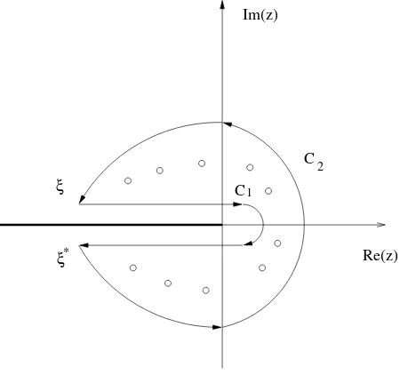
* Re(z)
Figure 4. Sketch of the integration contour. The open dots represent the rootsZj.
The situation is very similar to the one described in [38] for the one-species asymmetric exclusion model. Therefore we can adopt the technique to transform the discrete Bethe ansatz equations (14) to integral equations by using an identity that follows from the residue theorem:
1
In this equation,C is the contour enclosing all the rootsZj. We can view this contour C as
the union of two contoursC1 and C2 as shown in Fig.4.
These two contours intersect at two pointsξandξ⋆. We will fix those two points by requiring
YL(ξ⋆) =−π+
π
L, YL(ξ) =π− π L.
Rewriting this integral by separating the contributions coming from two contoursC1 andC2,
this becomes:
The formula for the energy reads:
E =L+ L
3
Conclusion and outlook
We have shown that the dynamical critical exponent of the totally asymmetric exclusion model is 32 which in the single-species asymmetric diffusion model is the exponent for the KPZ uni-versality class. This is a new result that cannot be deducted from the recent paper by Arita et al. [25].
The Bethe ansatz equations and their solutions are qualitatively very different from the case of a single species asymmetric exclusion model. It would be very interesting to derive this result analytically once the patterns of the solutions of the Bethe ansatz equations are fully understood. Building on the results reported here, the next step would be to solve the integral equations representing the Bethe ansatz equations in the continuum along the lines of de Gier and Essler [38]. Since the integration is performed over the curve formed by the roots in the thermodynamic limit, a qualitative understanding of this curve is a prerequisite for this calculation. We hope to report on this soon.
Another new direction will be to generalize the Bethe ansatz to the case of open boundaries.
Acknowledgements
We would like to thank V. Rittenberg for his continued interest and invaluable discussions and F.C. Alcaraz for sharing his manuscript about the Bethe ansatz with us. We would also like to acknowledge support from the Purdue Research Foundation.
References
[1] Ferrari P.A., Shocks in one-dimensional processes with a drift, in Probability and Phase Transition (Cam-bridge, UK, July 4–16, 1993), Editor G. Grimmett,NATO ASI Ser., Ser. C, Math. Phys. Sci., Vol. 420, Kluwer, Dordrecht, 1994, 35–48.
Ferrari P.A., Fontes L.R.G., Shock fluctuations in the asymmetric simple exclusion process,Probab. Theory Related Fields99(1994), 305–319.
[2] Derrida B., Lebowitz J.L., Speer E.R., Shock profiles for the asymmetric simple exclusion process in one dimension,J. Stat. Phys.89(1997), 135–167,cond-mat/9708051.
Bal´azs M., Microscopic shape of shocks in a domain growth model, J. Stat. Phys. 105 (2001), 511–524,
math.PR/0101124.
R´akos A., Sch¨utz G.M., Exact shock measures and steady-state selection in a driven diffusive system with two conserved densities,J. Stat. Phys.117(2004), 55–76,cond-mat/0401461.
B´alazs M., Farkas G., Kovacs P., R´akos A., Random walk of second class particles in product shock measures,
J. Stat. Phys.139(2010), 252–279,arXiv:0909.3071.
[3] Jafarpour F.H., Multiple shocks in a driven diffusive system with two species of particles, Phys. A 358 (2005), 413–422,cond-mat/0504093.
Jafarpour F.H., Masharian S.R., The study of shocks in three-states driven-diffusive systems: a matrix product approach,J. Stat. Mech. Theory Exp.2007(2007), P03009, 18 pages,cond-mat/0612622.
[4] Chowdhury A., Santen L., Schadschneider A., Statistical physics of vehicular traffic and some related systems,Phys. Rep.329(2000), 199–329,cond-mat/0007053.
[5] Macdonald J.T., Gibbs J.H., Pipkin A.C., Kinetics of biopolymerization on nucleic acid templates, Biopoly-mers6(1968), 1–25.
[6] Sch¨utz G., Non-equilibrium relaxation law for entangled polymers,Europhys. Lett.48(1999), 623–628. [7] Widom B., Viovy J.L., Defontaines A.D., Repton model of gel-electrophoresis and diffusion, J. Phys. I
France1(1991), 1759–1784.
[8] Dhar D., An exactly solved model for interfacial growth,Phase Transitions9(1987), 51–86.
[9] de Gier J., Essler F., Exact spectral gaps of the asymmetric exclusion process with open boundaries,J. Stat. Mech. Theory Exp.2006(2006), P12011, 46 pages,cond-mat/0609645.
[11] Gwa L.H., Spohn H., Bethe solution for the dynamical-scaling exponent of the noisy Burgers equation,Phys. Rev. A46(1992), 844–854.
[12] Sch¨utz G.M., Exact solution of the master equation for the asymmetric exclusion process,J. Stat. Phys.88 (1997), 427–445,cond-mat/9701019.
[13] Angel O., The stationary measure of a 2-type totally asymmetric exclusion process, J. Combin. Theory Ser. A113(2006), 625–635,math.PR/0501005.
[14] Evans M.R., Ferrari P.A., Mallick K., Matrix representation of the stationary mesure for the multispecies TASEP,J. Stat. Phys.135(2009), 217–239,arXiv:0807.0327.
[15] Ferrari P.A., Martin J.B., Stationary distributions of multi-type totally asymmetric exclusion processes,
Ann. Probab.35(2007), 807–832,math.PR/0501291.
[16] Prolhac S., Evans M.R., Mallick K., The matrix product solution of the multispecies partially asymmetric exclusion process,J. Phys. A: Math. Theor.42(2009), 165004, 25 pages,arXiv:0812.3293.
[17] Karimipour V., A multi-species asymmetric exclusion process, steady state and correlation functions on a periodic lattice,Europhys. Lett.47(1999), 304–310,cond-mat/9809193.
[18] Jafarpour F.H., A two-species exclusion model with open boundaries: a use of q-deformed algebra,
cond-mat/0004357.
[19] Evans M.R., Foster D.P., Godreche C., Mukamel D., Asymmetric exclusion model with two species: spon-taneous symmetry breaking,J. Stat. Phys.80(1995), 69–102.
Evans M.R., Foster D.P., Godreche C., Mukamel D., Spontaneous symmetry breaking in one dimensional driven diffusive system,Phys. Rev. Lett.74(1995), 208–211.
[20] Ayyer A., Lebowitz J., Speer E.R., On the two species asymmetric exclusion process with semi-permeable boundaries,J. Stat. Phys.135(2009), 1009–1037,arXiv:0807.2423.
[21] Uchiyama M., Two-species asymmetric exclusion process with open boundaries,Chaos Solitons Fractals35 (2008), 398–407,cond-mat/0703660.
[22] Arita C., Phase transitions in the two-species totally asymmetric exclusion process with boundaries,J. Stat. Mech. Theory Exp.2006(2006), P12008, 19 pages.
[23] Kim K.H., den Nijs M., Dynamic screening in a two-species asymmetric exclusion process,Phys. Rev. E76 (2007), 021107, 14 pages,arXiv:0705.1377.
[24] Arndt P.F., Heinzel T., Rittenberg V., Spontaneous breaking of translational invariance and spatial conden-sation in stationary states on a ring. I. The neutral system,J. Stat. Phys.97(1999), 1–65,cond-mat/9809123. [25] Arita C., Kuniba A., Sakai K., Sawabe T., Spectrum in multi-species simple exclusion process on a ring,
J. Phys. A: Math. Theor.42(2009), 345002, 41 pages,arXiv:0904.1481.
[26] Dahmen S.R., Reaction-diffusion processes described by three-state quantum chains and integrability,
J. Phys. A: Math. Gen.28(1995), 905–922,cond-mat/9405031.
[27] Popkov V., Fouladvand M.E., Sch¨utz G.M., A sufficient criterion for integrability of stochastic many-body dynamics and quantum spin chains,J. Phys. A: Math. Gen.35(2002), 7187–7204,hep-th/0205169. [28] Cantini L., Algebraic Bethe ansatz for the two-species ASEP with different hopping rates,J. Phys. A: Math.
Theor.41(2008), 095001, 16 pages,arXiv:0710.4083.
[29] Pr¨ahofer M., Spohn H., Current fluctuations for the totally asymmetric simple exclusion process, in In and Out of Equilibrium (Mambucaba, 2000), Editor V. Sidoravicius,Progr. Probab., Vol. 51, Birkh¨auser Boston, Boston, MA, 2002, 185–204,cond-mat/0101200.
B´alazs M., Sepp¨al¨ainen T., Exact connections between current fluctuations and the second class particle in a class of deposition models,J. Stat. Phys.127(2007), 431–455,math.PR/0608437.
[30] Alcaraz F.C., Droz M., Henkel M., Rittenberg, V., Reaction-diffusion processes, critical dynamics and quantum chains,Ann. Physics230(1994), 250–302,hep-th/9302112.
[31] Alcaraz F.C., Rittenberg, V., Reaction-diffusion processes as physical realizations of Hecke algebras,Phys. Lett. B314(1993), 377–380,hep-th/9306116.
[32] Kardar M., Parisi G., Zhang Y.C., Dynamic scaling of growing interfaces, Phys. Rev. Lett. 56 (1986), 889–892.
[33] Wilkinson D.R., Edwards S.F., The surface statistics of a granular aggregate,Proc. Roy. Soc. London Ser. A
381(1982), no. 1780, 33–51.
[34] Babelon O., de Vega H.J., Viallet C.-M., Exact solution of theZn+1×Zn+1symmetric generalization of the
[35] Alcaraz C., Lecture notes, unpublished.
[36] de Vega H.J., Yang–Baxter algebras, integrable theories and quantum groups,Internat. J. Modern Phys. A
4(1989), 2371–2463.
[37] Bulirsch R., Stoer J., Fehlerabsch¨atzungen und Extrapolation mit rationalen Funktionen bei Verfahren vom Richardson-Typus,Numer. Math.6(1964), 413–427.
Christe P., Henkel M., Introduction to conformal invariance and its applications to critical phenomena,
Lecture Notes in Physics, New Series m: Monographs, Vol. 16, Springer-Verlag, Berlin, 1993.