El e c t ro n ic
Jo ur n
a l o
f P
r
o ba b i l i t y
Vol. 6 (2001) Paper no. 3, pages 1–41. Journal URL
http://www.math.washington.edu/~ejpecp/ Paper URL
http://www.math.washington.edu/~ejpecp/EjpVol6/paper3.abs.html
LIMIT THEOREMS FOR THE NUMBER OF MAXIMA IN RANDOM SAMPLES FROM PLANAR REGIONS
Zhi-Dong Bai
Department of Statistics & Applied Probability, National University of Singapore, Singapore [email protected]
Hsien-Kuei Hwang1, Wen-Qi Liang and Tsung-Hsi Tsai Institute of Statistical Science, Academia Sinica, 115, Taiwan
[email protected], [email protected], [email protected]
AbstractWe prove that the number of maximal points in a random sample taken uniformly and inde-pendently from a convex polygon is asymptotically normal in the sense of convergence in distribution. Many new results for other planar regions are also derived. In particular, precise Poisson approximation results are given for the number of maxima in regions bounded above by a nondecreasing curve.
KeywordsMaximal points, multicriterial optimization, central limit theorems, Poisson approximations, convex polygons.
AMS subject classificationPrimary. 60D05; Secondary. 60C05
Submitted to EJP on September 29, 2000. Final version accepted on January 22, 2001.
1Part of the work of this author was done while visiting the Department of Statistics and Applied Probability, National
1
Introduction
A point p1 = (x1, y1) is said to dominate another point p2 = (x2, y2) if x1 ≥ x2 and y1 ≥ y2. For notational convenience, we write this asp1≻p2. Themaxima(or maximal points) of a sample of points are those points dominated by no other points in the sample. We investigate in this paper distributional properties of the number of maximal points in a random sample taken uniformly and independently from a given planar region.
Such a dominance relation (not restricted to planar points), known more frequently asPareto optimality, is an extremely useful notion in diverse fields ranging from economics to mechanics, from social sciences to algorithmics; see for example Karlin (1959), B¨uhlmann (1970), Leitman and Marzollo (1975), Preparata and Shamos (1985), Devroye (1986), Steuer (1986), Stadler (1988), Harsanyi (1988), Statnikov and Matusov (1995). It is one of the most natural order relations in multivariate observations because of the lack of intrinsic total order relations. Other terms like “efficiency” in econometrics, “noninferiority” in control, “admissibility” in statistics are all similar notions. One also finds a similar dominance relation used in a card game called “Russian poker.” From a probabilistic point of view, we do not distinguish in this paper the difference between>and≥, a key issue, however in other fields. The following quote from the review by J. Stoer and J. Zowe in AMS Mathematical Review (MR: 50 #3928) of Zeleny’s book [39] typically describes the general situation encountered in theory and practice:
One of the more pertinent criticisms of traditional decision-making theory and practice is directed against the approximation of multiple goal behavior by a single technical criterion. In a realistic model of a technical or economical optimization problem it will be impossible to tie all the given criteria into a single function, which could serve as objective function for an associated mathematical programming problem. It will be more appropriate to handle such problems as problems with a vector-valued objective function. Instead of finding an optimal solution of a single objective function, the problem is now one of locating the set of all nondominated points (also called efficient points or Pareto-optimal points).
We mention some concrete applications as follows.
1. Finding the maxima of a sample is a prototype problem with many algorithmic and practical ap-plications. Many geometric and graph-theoretic problems can be formulated as maxima-finding problems, including the problem ofcomputing the minimum independent dominating setin a per-mutation graph, the related problem of finding the shortest maximal increasing subsequence, the problem of enumerating restricted empty rectangles, and the related problem of computing the largest empty rectangle. Also the d-dimensional maxima-finding problem is equivalent to the en-closure problem for planar d-gon (where the corresponding sides are parallel), the latter problem in turn has several applications in CAD systems for VLSI circuits; see [16, 26, 33] for details and references.
2. The notion of dominance was used in Becker et al. (1987) to analyze data from the Places Rated Almanac, a collection of nine composite variables constructed for 329 metropolitan areas of the US. 3. The number of maxima is closely related to the performance of maxima-finding algorithms (Devroye (1986) and Preparata and Shamos (1985)); it was also used in probabilistic analysis of simplex algorithms in Blair (1986).
LetC be a given measurable region andMn(C) denote the number of maxima in a random sample ofn
points taken uniformly and independently fromC. Almost all results in the literature are concerned with the mean value ofMn(C). Distributional results are rare, the most studied case beingC= [0,1]2for which
the problem reduces to the number of records in iid (independent and identically distributed, here and throughout this paper) sequences of continuous random variables; see Baryshnikov (1987, 2000). From this connection, our study may also be regarded as another line of extensions of the theory of records; see R´enyi (1962), Barndorff-Nielsen and Sobel (1966), Arnold et al. (1998). The main contribution of this paper is to provide means of establishing the central limit theorem for Mn(C) when C is a convex
polygon and whenC is some region bounded above by a nondecreasing curve. Indeed, we derive precise Poisson approximation results in the second case (by computing the asymptotics of the total variation and Fortet-Mourier distances). A by-product of our central limit theorems gives the asymptotics of the variance. Many other auxiliary and structural results are also derived.
Results
Known results for Mn(C) when C = [0,1]d can be found in Bai et al. (1998), Devroye (1999) and the
references therein.
WhenC is a convex polygonP, Golin (1993) gave the following “gap theorem”:
E(Mn(P))≍
n1/2, logn, 1,
namely,E(Mn(P)) is either of ordern1/2, or of order logn, or bounded, and no other scales are possible.
On the other hand, Devroye (1993) showed that if
C={(x, y) : 0≤x≤1, 0≤y≤f(x)}, (1.1) wheref is nonincreasing and is eitherconvex, orconcave, orLipschitz (of order 1), then
E(Mn(C))∼π0n1/2, (1.2) where
π0=
π
2
1/2 R1
0 |f′(x)|1/2dx
R1
0 f(x) dx
1/2.
Note that by Cauchy-Schwarz inequality, it is easily deduced that the right-hand side of π0 reaches its maximal value whenC is a right triangle with decreasing hypotenuse of the shape ❅❅; compare Dwyer (1990).
Our first result shows in a precise way that in the case of a convex polygonP E(Mn(P)) =π1n1/2+π2logn+π3+O(n−1/2),
where π1 is essentially Devroye’s (“discretized”) constant, π2 can assume only values 0,1/2 and 1, and π3 is a complicated constant; see (1.3), (1.6), (3.9) and (3.12) for explicit expressions of these constants. More precisely, let
y∗= sup{y : (x, y)∈ P}, x∗= sup{x : (x, y)∈ P}, and then define
Iu={(x, y∗) : (x, y∗)∈ P}, Ir={(x∗, y) : (x∗, y)∈ P}.
In words, if we move a horizontal line from∞downwards, thenIudenotes the intersection of this line and
P when they first meet; likewise,Ir denotes the intersection of a vertical line moving from∞ leftwards
Theupper-right partofP is defined as
P ∩ {(x, y) : x≥minIu, y≥minIr},
where minIu := min{x : (x, y∗)∈ P} and minIr := min{y,: (x∗, y)∈ P}. Note that the upper-right
part can be either a point, or one or two lines, or a region with nonzero measure. Also note that this definition applies to any other planar regions.
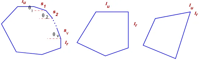
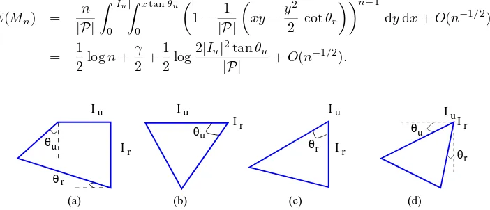
Define s1, s2, . . . , sν to be the line segments on the upper-right part ofP which bridge Iu andIr when
Iu∩Ir=∅, where∅ denotes the empty set. Also let θj be the angle formed bysj and a horizontal line
forj= 1, . . . , ν; see Figure 1 for an illustration.
θ
θ
s
s
s
u 2
u 1
ν
θ u
r
r
1
ν 2
I
I
I
I
I
[image:4.612.134.465.221.321.2]Ir
Figure 1: Possible configurations of convex polygons.
LetN(0,1) denote a normal random variable with zero mean and unit variance. Let|P|and|sj|denote
the area and length, respectively, ofP andsj.
Theorem 1 (CLT for convex polygons). The mean of Mn(P)satisfies
E(Mn(P)) =π1n1/2+π2logn+π3+O
(ν+ 1)n−1/2, (1.3)
where
π1 =
π 2|P|
1/2 X
1≤j≤ν
|sj|(cosθjsinθj)1/2. (1.4)
π2 = 1
2 1{|Iu|>0}+ 1{|Ir|>0}
∈ {0,1/2,1}, (1.5)
andπ3 is given in (3.9) and (3.12). If in additionIu∩Ir=∅ (π1>0), then
Var(Mn(P))∼σ12n1/2, (1.6)
and
Mn(P)−π1n1/2 σ1n1/4
D
−→ N(0,1), (1.7)
whereσ1= (π1(2 log 2−1))1/2 and
D
−→ denotes convergence in distribution. Ifπ1= 0 andπ2>0 then
Var(Mn(P))∼π2logn, (1.8)
and
Mn(P)−π2logn (π2logn)1/2
D
The proof of (1.7) consists in first splitting the upper-right part ofP that lies inP into triangles of the form (except possibly the first and the last). Thus the asymptotic normality of Mn(P) is reduced
to that of Mn(T), where T is the right triangle with corners (0,0), (0,1) and (1,0). It turns out that
in this specific case,Mn(T) enjoys many interesting properties; details are examined in the next section.
Originally, our proof for the asymptotic normality ofMn(T) proceeded by computing the third and fourth
central moments, which was very laborious; see Bai et al. (2000) for details. The proof given here uses the method of moments, and, because of a better manipulation of the recurrence, the result is stronger (convergence of all moments) and the proof is much shorter. The proof of Theorem 1, except (1.8) and (1.9), is then given in Section 3. The case whenIu∩Ir6=∅ is essentially a special case of Theorem 2; a
sketch of proof is given in Section 6. Note that in the special case whenP is the unit square, the result (1.9) can be easily proved by checking Lyapunov’s condition.
Our proof actually covers the case when the underlying regionP is not convex, provided that the upper-right part ofP can be split into a finite union of triangles and rectangles; see Section 3.2.
A comparison of (1.3) with the result for the expected number of points on the convex hull ofniid points chosen uniformly fromP by R´enyi and Sulanke (1963) shows that there are considerably more maxima than hull points in a random sample whenIu∩Ir=∅(the former can be used to approximate the latter;
see Devroye, 1980). For more information on related results, see Buchta and Reitzner (1997) and the references given there.
The surprising factor 1/2 in (1.3) and (1.5) suggests several new questions like “Why it is 1/2?” “Is this factor universal?”, and “Since this factor depends (from (1.5)) only on the boundary of the upper-right part ofP, what happens for general regions?”
It is for answering these questions that we study the following two problems. First, if we compare (1.2) and (1.3), it is then natural to consider the convergence rate of Devroye’s result (1.2). Devroye (1993) observed that the continuous part off′ contributes then1/2 term (as in the expression ofπ0), while the discontinuous points contributeO(logn) maximal points on average. We show that iff is piecewise twice continuously differentiable then the next dominant term in (1.2) is asymptotic toclogn, wherec can be explicitly computed in terms of the local behaviors off near “critical points,” that is, points at which |f′| = 0, or |f′| = ∞ or f′ does not exist. This result thus connects the critical points and the logn
term in the asymptotic expression ofE(Mn) in a quantitatively precise way. The idea is to breakf at all
critical points and then to sum over the expected number of maxima (scaled by their area proportions) in each smaller regions with more smooth boundaries (see Figure 8), the hard part being the determination of the coefficient of the log term. This problem is discussed in Section 4.
Second, we consider E(Mn(C)) when C is bounded by two nondecreasing curves. We show that if the
rates that the two functions tend to their values at unity are the same thenE(Mn(C)) is asymptotic to a
constant; otherwise, it is asymptotic toclognfor some constantc. In particular, if one curve is linear and the other is either a vertical or horizontal line, then c= 1/2. This consideration thus partly interprets the constant 1/2 in a deeper way.
The last problem we consider is the distribution of Mn(C) when C is of the shape (1.1), where f is
nondecreasing. It is well known that whenf(x)≡1,Mn is well approximated by a Poisson distribution
with mean logn[29]. We derive, under suitable conditions on f, precise asymptotic approximations for the total variation and Fortet-Mourier distances between the distribution ofMn(C) and a suitable Poisson
distribution. Actually, our results suggest that Poisson law (with bounded or unbounded mean) is the
universal limit law of Mn for nondecreasing f; see the discussion in Section 6 for more support of this
suggestion.
defined, respectively, by
dTV(L(X),L(Y)) = 1 2
X
j≥0
|P(X=j)−P(Y =j)|,
dFM(L(X),L(Y)) = X
j≥0
|P(X ≤j)−P(Y ≤j)|.
Theorem 2 (Poisson approximation). Assume thatf is nondecreasing,R1
0 f(t) dt= 1 and xf(1−x)
1−F(1−x) = 1−(1−F(1−x))
α(a+L(1
−F(1−x))),
wherea, α >0,F(x) :=Rx
0 f(t) dt, and
L(x) =O |logx|−1
, (1.10)
asx→0+. Then the mean and the variance ofM
n satisfy
E(Mn) = α
α+ 1logn+
αγ−loga
α+ 1 +O (logn)
−1
,
Var(Mn) =
α
α+ 1logn+
(6γ−π2)α2+ (6γ −2π2
−6 loga)α−6 loga 6(α+ 1)2
+O (logn)−1
, (1.11)
whereγ is the Euler constant. Furthermore, the distribution ofMn is asymptotically Poisson:
dTV(L(Mn),L(Y)) = √ κ
2πe λ
1 +O(logn)−1/2, dFM(L(Mn),L(Y)) = √κ
2πλ
1 +O(logn)−1/2,
whereY is a Poisson variate with mean λ=αα+1logn+αγα−+1loga−1:
P(Y =m) =e−λ λ
m−1
(m−1)!, (m≥1),
and
κ=
1−π
2α(α+ 2) 6(α+ 1)2
.
In particular,Mnis asymptotically normally distributed with mean and variance asymptotic to αα+1logn.
We can indeed derive a local limit theorem forMn.
Note that
κ=±
1−π
2α(α+ 2) 6(α+ 1)2
,
depending on α <−1 +π/√π2−6 (plus sign) or α > −1 +π/√π2−6 (minus sign). The case when α=−1 +π/√π2−6 is of special interest sinceκ= 0 and our result reduces to an upper estimate. If we replace (1.10) in this case byL(x) =O |logx|−3/2
, then we can show, using the proof techniques for Theorem 2 and the approach in [29], that
dTV(L(Mn),L(Y)) =
κ1 3√2π
4e−3/2+ 1λ−3/21 +O(logn)−1/2,
dFM(L(Mn),L(Y)) = 2
√ 2κ1 3√πeλ
whereκ1=ζ(3)(π2−6)3/2/π3−ζ(3) + 1,ζ(3) =Pj≥1j−3.
The proof of Theorem 2 relies on an explicit expression for the moment generating function (in terms of moment generating function ofMn(C) whenC is a rectangle) and a careful analysis of the associated
sums and integrals. Details as well as other Poisson approximation results are given in Section 6. Notation. Throughout this paper,nis the major asymptotic parameter which is taken to be sufficiently large. All limits, whenever unspecified, is taken to ben→ ∞. The generic symbolsε, c, andK always represent suitably small, absolute, and large, respectively, positive constants independent of n whose values may vary from one occurrence to another. The symbol [zn]F(z) denotes the coefficient of zn in
the Taylor expansion ofF(z). We write simplyMn when there is no ambiguity of the underlying planar
region.
2
Maxima in right triangles
LetT denote the right triangle with corners (0,0), (0,1) and (1,0). We prove in this section the asymptotic normality of Mn = Mn(T) by the method of moments. The key idea of the proof is to compute the
(centralized) moments recursively and then to reduce all major asymptotic estimates to an asymptotic transfer lemma (see Lemma 4).
Theorem 3 (CLT for triangle). The mean and the variance of Mn satisfy
E(Mn) =
√πn!
Γ(n+ 1/2) −1 (2.1)
= √πn−1 + √π 8√n+
√π 128n3/2 +O
n−5/2,
Var(Mn) = πn−
π n!2 Γ(n+ 1/2)2 +
√πn!
Γ(n+ 1/2)(2 log 2−1) +O n
−K
(2.2)
= σ22 √
n−π4 + σ 2 2 8√n−
π 32n+
σ2 2 128n3/2+
π 128n2+O
n−5/2,
for anyK >0, whereσ2= (2 log 2−1)1/2π1/4. The distribution of(Mn−√πn)/(σ2n1/4)is asymptotically
normal:
Mn−(πn)1/2
σ2n1/4
D
−→ N(0,1), (2.3)
where the limit holds with convergence of all moments.
2.1
Moment generating function
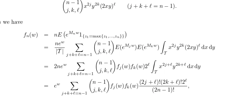
Proposition 1. The moment generating functionfn(w) :=E(eMnw) ofMn satisfies the recurrence
fn(w) =ew X
j+k+ℓ=n−1
πj,k,ℓ(n)fj(w)fk(w), (2.4)
for n ≥1 with the initial condition f0(w) = 1, where the sum is extended over all nonnegative integer triples (j, k, ℓ)such that j+k+ℓ=n−1 and
πj,k,ℓ(n) :=
n−1 j, k, ℓ
2ℓ
Z 1
0
x2j+ℓ(1−x)2k+ℓdx=
n−1 j, k, ℓ
(2j+ℓ)!(2k+ℓ)!2ℓ
0000 0000 1111 1111 00000 00000 00000 00000 00000 11111 11111 11111 11111 11111
T R
(x,y) T
no maxima here
no points here
1,x,y
[image:8.612.91.489.310.486.2]x,y 2,x,y
Figure 2: Division of the original right triangle at the point wherexj+yj is maximized; the number of
maxima is thus computed recursively.
Proof.LetXj = (xj, yj),j = 1, . . . , n, ben iid points taken uniformly inT. Letzj=xj+yj.
The idea of the proof is to find the point, sayX1, that maximizes the sumxj+yj, writing for simplicity
X1= (x, y); and then to divide the triangle into two smaller triangles,T1,x,y andT2,x,y, and a rectangle
Rx,y, as shown in Figure 2. Since the rectangleRx,y contains no maxima, the number of maxima Mn
inT equals 1 plus those in the two smaller triangles. The probability that there arej points inT1,x,y,k
points inT2,x,y andℓ points in the rectangleRx,y is equal to n
−1 j, k, ℓ
x2jy2k(2xy)ℓ (j+k+ℓ=n−1).
Thus we have
fn(w) = nE eMnw1{z1=max{z1,...,zn}}
= ne
w
|T |
X
j+k+ℓ=n−1
n−1 j, k, ℓ
E(eMjw)E(eMkw)
Z
T
x2jy2k(2xy)ℓdxdy
= 2new X
j+k+ℓ=n−1
n−1 j, k, ℓ
fj(w)fk(w)2ℓ Z
T
x2j+ℓy2k+ℓdxdy
= ew X
j+k+ℓ=n−1
n
−1 j, k, ℓ
fj(w)fk(w)
(2j+ℓ)!(2k+ℓ)!2ℓ
(2n−1)! ,
from which (2.4) follows.
A “random divorce model?” The above probability distribution has a straightforward probabilistic interpretation: Givenn−1 couples, we randomly divide them into two groups with sizestand 2n−2−t, where 0 ≤ t ≤2n−2. Then πj,k,ℓ(n) is the probability that there are j couples in one group and k
couples in the other, the number of “un-coupled” beingℓ = t−2j = 2n−2−t−2k in both groups. From this point of view, the number of maxima in T can also be interpreted as the total number of steps needed to completely “divorce”n−1 couples by repeating the above procedure until no further such divisions are possible, namely, when the sizes of all subproblems (or number of couples) reduce to zero. Our result (2.3) is equivalent to saying that this quantity is asymptotically normally distributed; see Frieze and Pittel (1995) for a similar example.
LetG(z, w) =e−zP
n≥0fn(w)zn/n!. ThenGis entire inz satisfyingG(0, w) = 1 and
∂
∂zG(z, w) +G(z, w) =e
w Z 1
0
G(x2z, w)G((1
2.2
Mean and variance
We prove (2.1) and (2.2). Taking derivative on both sides of (2.6) with respective towand substituting w= 0, we obtainG1(0) = 0 and
G′
1(z) +G1(z) = 1 + 2
Z 1
0
G1(x2z) dx, where G1(z) = (∂/∂w)G(z, w)
w=0. Write G1(z) = P
n≥0g1(n)zn. Then g1(0) = 0 and by equating coefficient ofzn on both sides
(n+ 1)g1(n+ 1) +g1(n) =δn0+ 2g1(n)
2n+ 1 (n≥0), whereδabis the Kronecker symbol. Solving this recurrence, we have
g1(n) =
(−1)n−1
(2n−1)n! (n≥1). Thus the mean ofMn is equal to
E(Mn) =n![zn]ezG1(z) =
X
1≤j≤n n
j
(
−1)j−1 2j−1 =
√πn!
Γ(n+ 1/2)−1 = 4n
2n n
−1.
This proves (2.1). The asymptotic approximation ofE(Mn) follows from Stirling’s formula. Note that
(2.1) can be proved in a more straightforward way by computing the probability that a point is maximal. Taking derivative twice with respect towand substituting w= 0 in (2.6), we obtainG2(0) = 0 and
G′
2(z) +G2(z) = 1 + 2
Z 1
0
G2(x2z) dx+ 4
Z 1
0
G1(x2z) dx+ 2
Z 1
0
G1(x2z)G1((1
−x)2z) dx, whereG2(z) = (∂2/∂w2)G(z, w)
w=0. Write G2(z) = P
n≥0g2(n)zn. We haveg2(0) = 0 and (n+ 1)g2(n+ 1) +g2(n) =δn0+4g1(n)
2n+ 1 + 2
X
0≤j≤n
g1(j)g1(n−j)
(2j)!(2n−2j)! (2n+ 1)! +
2g2(n) 2n+ 1, forn≥0. Solving the recurrence, we obtain
g2(n) =
(−1)n−1 (2n−1)n! +
X
0≤j≤n−2
(−1)j(n
−j)!(2n−2j−1)
(2n−1)n! g11(n−j), where
g11(n) =
4g1(n−1) n(2n−1) +
2 n(2n−1)!
X
0≤ℓ≤n−1
g1(ℓ)g1(n−1−ℓ)(2ℓ)!(2n−2ℓ−2)!. Thus the second moment ofMn satisfies forn≥1
E(Mn2) = n![zn]ezG2(z) = E(Mn) +
X
2≤m≤n n
m
(
−1)m
2m−1
X
2≤j≤m
(−1)jj!(2j
−1)g11(j)
= E(Mn) + 4 X
2≤m≤n
n m
(−1)m
2m−1
X
0≤j≤m−2 1 2j+ 1
+ 2 X 3≤m≤n
n m
(−1)m−1 2m−1
X
0≤j≤m−3
1 (2j+ 1)(2j+ 3)
X
0≤ℓ≤j j ℓ 2j 2ℓ
To derive asymptotics ofE(M2
n), since both sums Σ1,Σ2 are of the type P
n0≤j≤n
n j
(−1)ja
j for some
sequenceaj, which can essentially be regarded as then-th difference ofa0, we use the associated integral
representation from finite differences to evaluate the sums; see [23]. Lemma 1. The sumsΣ1 andΣ2 satisfy the asymptotic expansions
Σ1 ∼ 2
√π n!
Γ(n+ 1/2)(ψ(n+ 1/2) +γ−2) + 4 +
X
j≥0
Γ(j+ 1/2)n!
Γ(n+j+ 3/2)(j+ 1), (2.7) Σ2 ∼ πn− 2
√πn!
Γ(n+ 1/2)(ψ(n+ 1/2)−log 2 +γ)−2−
X
j≥0
Γ(j+ 1/2)n!
Γ(n+j+ 3/2)(j+ 1), (2.8)
whereψ denotes the logarithmic derivative of the Gamma function.
Proof.Observe that the functionφ1(s) :=ψ(s−1/2)/2 +γ/2 + log 2 satisfies form≥2 φ1(m) = X
0≤j≤m−2 1 2j+ 1. Thus we have [23]
Σ1= 4 2πi
Z 3/2+i∞
3/2−i∞
(−1)n+1n!φ1(s)
s(s−1)· · ·(s−n)(2s−1)ds.
Since the growth rate ofψ(s) atσ±i∞is of logarithmic order, we can evaluate the integral by shifting the line of integration to the left and by taking the residues of the poles encountered into account. There is no pole ats= 1 because φ1(1) = 0. The only singularities are (i) a double pole at s= 1/2 and (ii) simple poles at s= 0 and s=−1/2−j forj ≥0. Collecting the residues of these poles, we obtain the asymptotic expansion (2.7).
Similarly, define forℜ(s)>1
φ2(s) =X
j≥0
1 2j+ 3
Z 1
0
ω(x)jdx− 1 2j+ 2s−1
Z 1
0
ω(x)j+s−2dx
,
whereω(x) := 1−2x+ 2x2. Then
Σ2= 2 2πi
Z 5/2+i∞
5/2−i∞
(−1)nn!φ2(s)
s(s−1)· · ·(s−n)(2s−1)ds.
It is easy to show that φ2(σ±iT) = O(1) for large T > 1. Note that φ2(2) = 0. We are left with the calculation of the residues at the (i) double pole at s = 1/2 and (ii) simple poles at s = 1,0 and s=−j−1/2 forj≥0. We need the following identities
Z 1
0
ω(x)−1dx=π 2,
Z 1
0
ω(x)−3/2dx= 2,
Z 1
0
ω(x)−2dx= 1 +π 2. ¿From these it follows thatφ2(1) =−π/2,φ2(0) = 1, and
φ2(s) = − 1
s−1/2 +c1+O(|s−1/2|) (s∼1/2), φ2(s) = − 1
where
c1 =
X
j≥0 1 2j+ 3
Z 1
0
ω(x)jdx−12
Z 1
0
logω(x) ω(x)3/2 dx−
X
j≥1 1 2j
Z 1
0
ω(x)j−3/2dx
= −π2 + 2
Z 1/2
0
ω(x)−3/2log1 +
p
ω(x)
p
ω(x) dx = 3 log 2−2.
Collecting residues from the integral representation of Σ2, we obtain (2.8).
Noting that there are perfect cancellations of theψ-terms and the last sums in both expansions (2.7) and (2.8), we obtain
E(Mn2) =E(Mn) + Σ1+ Σ2=πn+
√πn!
Γ(n+ 1/2)(2 log 2−3) + 1 +O n
−K
,
for anyK >0. This completes the proof of (2.2) for the variance ofMn.
2.3
Higher moments
We prove in this section that form≥1
E Mn−√πn
2m
∼ hmnm/2, (2.9)
E Mn−√πn 2m−1
= onm/2−1/4, (2.10) where hm := (2m)!σ22m/(2mm!). From these the asymptotic normality of (Mn −√πn)/(σ2n1/4) will follow.
The casem= 1 holds by (2.1) and (2.2). We prove the remaining casesm≥2 by induction. A different approach for the asymptotics of higher moments is needed since the preceding one becomes too involved for moments of degree≥3; see Bai et al. [4].
Shifting the mean. LetPn(w) :=E(e(Mn−
√πn)w
) =fn(w)e−
√πnw
. ThenP0(w) = 1 and, by (2.4), Pn(w) =
X
j+k+ℓ=n−1
πj,k,ℓ(n)Pj(w)Pk(w)e∆n,j,kw (n≥1), (2.11)
where ∆n,j,k:=√πj+
√
πk−√πn+ 1. DefinePn,m:=Pn(m)(0) =E(Mn−√πn)m.
Lemma 2. The sequencesPn,m satisfy the recurrenceP0,m= 0, P1,m = (1−√π)m and forn≥2 and
m≥1
Pn,m=
(n−1)! Γ(n+ 1/2)
X
0≤j<n
Γ(j+ 1/2)
j! Pj,m+R (1)
n,m+R(2)n,m, (2.12)
where
R(1)n,m := X
1≤p<m
m p
X
j+k+ℓ=n−1
πj,k,ℓ(n)Pj,pPk,m−p,
R(2)n,m :=
X
p+q+r=m
0≤p,q<m
1≤r≤m m
p, q, r
X
j+k+ℓ=n−1
Proof.By (2.11),
Pn,m =
X
p+q+r=m
m p, q, r
X
j+k+ℓ=n−1
πj,k,ℓ(n)Pj,pPk,q∆rn,j,k
= X
j+k+ℓ=n−1
πj,k,ℓ(n) (Pj,m+Pk,m) +R(1)n,m+R(2)n,m
= 2 X
j+k+ℓ=n−1
πj,k,ℓ(n)Pj,m+R(1)n,m+R(2)n,m.
Now, by the integral representation in (2.5), we have
2 X
j+k+ℓ=n−1
πj,k,ℓ(n)Pj,m
= 2 X
0≤j<n n
−1 j
Pj,m Z 1
0 x2j(1
−x)n−1−j X
0≤k<n−j n
−1−j k
(2x)n−1−j−k(1
−x)kdx
= 2 X
0≤j<n
n−1 j
Pj,m Z 1
0
x2j(1−x2)n−1−jdx.
The recurrence (2.12) follows.
Solution and asymptotic transfers of the recurrence. We first study recurrences of the type (2.12).
Lemma 3. Assumea0= 0 and an =
(n−1)! Γ(n+ 1/2)
X
0≤j<n
Γ(j+ 1/2)
j! aj+bn (n≥1), (2.13)
wherebn is a given sequence. Then for n≥1
an =bn+ n!
Γ(n+ 1/2)
X
0≤j<n
Γ(j+ 1/2)
(j+ 1)! bj. (2.14)
Proof.Define ˜an = Γ(n+ 1/2)an/n! and ˜bn= Γ(n+ 1/2)bn/n!. Then ˜a0= 0 and ˜
an=
1 n
X
0≤j<n
˜
aj+ ˜bn (n≥1).
By considering the differencen˜an−(n−1)˜an−1 and iterating, we obtain
˜
an = ˜bn+ X
1≤j<n
˜ bj
j+ 1 (n≥1),
which yields (2.14).
Lemma 4 (Asymptotic transfer). Assume thatan satisfies (2.13) and thatα > 1/2. If bn ∼cnα,
then
an ∼c
2α+ 1 2α−1n
α; (2.15)
ifbn=O(nα), orbn =o(nα), thenan=O(nα), oran=o(nα), respectively.
Proof.By (2.14).
By (2.12) and the asymptotic transfer lemma, the proofs of (2.9) and (2.10) are reduced, by induction, to estimating the asymptotics ofR(1)n,mandR(2)n,m.
Asymptotics of Rn,m(1) . By (2.9), (2.10) and induction, we have for m≥2
Rn,(1)2m−1 = X 1≤p≤2m−2
2m
−1 p
X
j+k+ℓ=n−1
πj,k,ℓ(n)Pj,pPk,2m−1−p
= o
X
1≤p≤2m−2
2m
−1 p
X
j+k+ℓ=n−1
πj,k,ℓ(n)jp/4k(2m−1−p)/4
= onm/2−1/4. (2.16)
On the other hand,
R(1)n,2m = X 1≤p<m
2m
2p
X
j+k+ℓ=n−1
πj,k,ℓ(n)Pj,pPk,2m−p+o(nm/2)
∼ X
1≤p<m 2m
2p
hphm−pUm,p(n),
where
Um,p:= X
j+k+ℓ=n−1
πj,k,ℓ(n)jp/2k(m−p)/2.
By (2.5)
Um,p(n)n−m/2 = Z 1
0
X
j+k+ℓ=n−1
n
−1 j, k, ℓ
x2j(1−x)2k[2x(1−x)]ℓ(j/n)p/2(k/n)(m−p)/2dx
:=
Z 1
0
Eh(J/n)p/2(K/n)(m−p)/2idx,
where (J, K,Λ) denotes a trinomial distribution with parameters (n−1;x2,(1
−x)2,2x(1 −x)). By Bernstein’s inequality, we have, uniformly inxand for sufficiently largen,
P
J/n−x2
≥n−1/3 h
n−7/12∨x(1−x)i ≤ 2 exp
−15minnn1/3, n2/3hn−7/12∨x(1−x)io
≤ 2 exp
−15n1/12
and, similarly, P
K/n−(1−x)2
≥n−1/3 h
n−7/12∨x(1−x)i≤2 exp
−15n1/12
.
When|J/n−x2
| ≤n−1/3x(1
−x),|K/n−(1−x)2
| ≤n−1/3x(1
−x) andn−1/3< x <1
−n−1/3, we have
(J/n)
p/2(K/n)(m−p)/2 −xp(1
−x)(m−p)/2 ≤ p
p
J/n−x
+ (m−p)
p
K/n−(1−x)
= p|J/n−x 2
|
p
J/n+x +
(m−p)|K/n−(1−x)2 |
p
K/n+ (1−x) ≤ mn−1/3.
Thus,
Um,p(n)n−m/2 =
Z 1−n−1/3 n−1/3
xp(1
−x)m−pdx+O(n−1/3)
= p!(m−p)! (m+ 1)! +O(n
−1/3). Consequently,
R(1)n,2m∼
nm/2 m+ 1
X
1≤p<m
2m
2p
m p
hphm−p=
m−1 m+ 1hmn
m/2. (2.17)
Estimate forR(2)n,m. We use a slightly different method to estimateRn,m(2) since there are additional
can-cellations caused by the factor ∆r
n,j,k. Denote again by (J, K,Λ) a trinomial distribution with parameters
(n−1;x2,(1
−x)2,2x(1
−x)). By induction, (2.9) and (2.10), we have R(2)n,m=
X
p+q+r=m
0≤p,q<m
1≤r≤m m
p, q, r
On(m+r)/4Vr(n),
where
Vr(n) := n−r/2 X
j+k+ℓ=n−1
πj,k,ℓ(n)|∆j,k(n)|r
= Z 1 0 E p
πJ/n+pπK/n−√π+n−1/2 r
dx.
By an argument similar to the estimate ofUm,p(n) using Bernstein’s inequality, we have
p
πJ/n+pπK/n−√π+n−1/2 r
=o(n−r/4), for|J/n−x2
| ≤n−1/3
n−7/12
∨x(1−x)
and|K/n−(1−x)2
| ≤n−1/3
n−7/12
∨x(1−x)
. Also P
J/n−x2
≥n−1/3 h
n−7/12∨x(1−x)i ≤ 2e−n1/12/5 PK/n−(1−x)2
≥n−1/3 h
n−7/12∨x(1−x)i ≤ 2e−n1/12/5. Thus
Vr(n) =o(n−r/4) +O
from which it follows that
R(2)n,m=o(nm/4). (2.18)
An alternative way of estimatingVr(n) is as follows. Using the inequality |x| ≤ex+e−xfor x∈R, we have
Vr(n)nr/2≤ X
j+k+ℓ=n−1
πj,k,ℓ(n) er∆n,j,k+e−r∆n,j,k
=:Vr+(n) +Vr−(n).
LetW(z) :=P j≥0er
√
πjzj/j!. Then
Vr+(n) =er(1−
√
πn)(n
−1)![zn−1]
Z 1
0
W(x2z)W((1−x)2z)e2x(1−x)zdx.
By the local limit theorem for Poisson distribution (or the saddlepoint method), we have W(y) =Oey+r√πy (y→ ∞).
Using Cauchy’s integral formula and this estimate, we obtain
Vr+(n) ≤ er(1−
√πn)
(n−1)! 2πi
I
|z|=n
z−n
Z 1
0
W(x2z)W((1−x)2z)e2x(1−x)zdxdz
≤ er(1−√πn)(n−1)! 2π n
1−nZ π
−π Z 1
0
W(x2n)W((1−x)2n)e2x(1−x)ncosθdxdθ
= O
n!n−nenZ
1 0
Z π
−π
e−2x(1−x)n(1−cosθ)dθdx
.
By the inequality 1−cosθ≥2θ2/π2 for|θ| ≤π, we have
V+
r (n) =O
n!n−nenn−1/2
Z 1
0
x−1/2(1
−x)−1/2dx
=O(1).
Similarly,V−
r (n) =O(1). ThusVr(n) =O(n−r/2) and (2.18) follows.
Asymptotics of Pn,m. By the estimates (2.16), (2.17) and (2.18), we obtain
R(1)n,2m+R(2)n,2m ∼ m−1 m+ 1 ×
(2m)! 2mm!σ
2mnm/2
R(1)n,2m−1+R (2)
n,2m−1 = o
nm/2−1/4,
form≥2. The results (2.9) and (2.10) follow then from applying the asymptotic transfer lemma. This
completes the proof of (2.3) and Theorem 3.
3
Maxima in convex polygons
3.1
Mean value of
M
n(
P
)
We prove (1.3) in this section. Our approach can actually provide an asymptotic expansion but we content ourselves with (1.3) for simplicity.
LetX1, . . . , Xn be iid random variables uniformly distributed inP. For A ⊂ P, denote by Mn(A) the
number of maxima of the point set{X1, . . . , Xn}lying inA. Also writeMn=Mn(P).
Observe first that forA ⊂ P
E(Mn(A)) = nP{X1∈ Aand is a maximal point of{X1, . . . , Xn}}
= n
|P|
Z
A
1−|P ∩ {s : s≻t}| |P|
n−1
dt. (3.1)
The following lemma is useful for estimating Laplace-type integrals encountered in this paper. Lemma 5. For0≤t≤1 andn≥1, the inequalities
e−nt 1−nt2
≤(1−t)n≤e−nt (3.2)
hold.
Proof.The right inequality is obvious. For the left inequality, we have e−nt−(1−t)n = e−nt 1− et(1−t)n
≤ e−nt 1−(1−t2)n
≤ e−ntnt2, by using the inequalitieset
≥1 +tand (1−t)n
≥1−nt(by induction).
Most Laplace integrals in this paper are of the type
Z 1
0
1−T(x) (1 +O(E(x)))n−1dx,
for someT andE. If we apply the above lemma and the inequality|et−1| ≤tet, we obtain Z 1
0
1−T(x) (1 +O(E(x)))n−1dx=
Z 1
0
e−nT(x) 1 +O T(x) +nT2(x) +nE(x)
dx,
which is usually easier to deal with than a “microscopic analysis”.
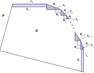
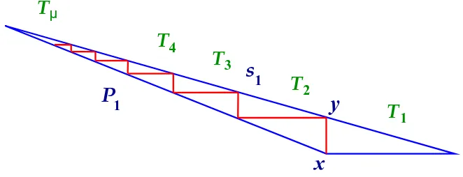
Case 1: Iu∩Ir=∅. LetPj be the right triangle with hypotenusesj (and undersj), the angle formed
bysj and the adjacent beingθj(see Figure 3). Note that part ofPj may lie outsideP (see Figure 4(b)).
Lemma 6. IfPj⊂ P, then
E(Mn(Pj)) =
|Pj|πn
|P|
1/2
−1 +On−1/2, (3.3)
000 000 000 000 000 000 000 000 000 000 000 000 000 000 000 000 000 000 000 000 111 111 111 111 111 111 111 111 111 111 111 111 111 111 111 111 111 111 111 111 0000000000000000000000000000000 0000000000000000000000000000000 0000000000000000000000000000000 1111111111111111111111111111111 1111111111111111111111111111111 1111111111111111111111111111111 ν ν ν −1 −1 u 1 r r θ
θν−1
[image:17.612.137.462.91.344.2]θν θ3 2 1 R P R P R Z P u 1 2 3 2 P P Z θ I I
P
D
Figure 3: Dissection of the upper-right part of a convex polygon P.
Proof.By (3.1) and the integral representation for finite differences [23], we have
E(Mn(Pj)) =
n |P|
Z |sj|cosθj 0
Z xtanθj 0
1−cotθj 2|P| y
2
n−1 dydx
= X
1≤k≤n n
k
(−1)k−1(|Pj|/|P|)k
2k−1
= 1
2πi
Z 3/4+i∞
3/4−i∞
(−1)nn!(
|Pj|/|P|)s
s(s−1)· · ·(s−n)(2s−1)ds = (|Pj|/|P|)
1/2√π n!
Γ(n+ 1/2) −1 +O n
−K
,
for anyK >0. The formula (3.3) follows.
Let Rj be a rectangle between Pj andPj+1 as shown in Figure 3 (the exact position of the lower-left boundary ofRj being immaterial).
Lemma 7. Forj = 1, . . . , ν−1,
E(Mn(Rj)) =
p
tanθj+1 2p
tanθj+1−tanθj
log
p
tanθj+1+ptanθj+1−tanθj p
tanθj+1−ptanθj+1−tanθj
+O(n−K), (3.4)
Proof.By (3.1) and a change of variables, we have
E(Mn(Rj)) =
n |P| Z ε 0 Z ε 0
1− 1 |P|
tanθ j
2 x
2+xy+cotθj+1
2 y
2
n−1
dydx+O(n−K)
= n |P| Z ε 0 Z ε/x 0 x
1− x 2 2|P|ζ(y)
n−1
dydx+O(n−K),
for anyK >0, whereζ(y) = tanθj+ 2y+y2cotθj+1. Interchanging the order of integration, the first
term on the right-hand side is equal to
Z 1
0
ζ(y)−1
1−
1−ε 2ζ(y) 2|P|
n
dy+
Z ∞
1
ζ(y)−1
1−
1−ε 2ζ(y) 2|P|y2
n
dy
=
Z ∞
0
ζ(y)−1dy+O(n−K),
from which (3.4) follows.
Note that when θj+1 → θj, E(Mn(Rj)) → 1, which cancels nicely with the constant in (3.3); this is
consistent with the result (2.1) forT.
LetZu,Zr be the trapezoids formed byIu andIr, respectively, as shown in Figure 3 when |Iu|>0 and
|Ir|>0.
Lemma 8. If|Iu|>0 then
E(Mn(Zu)) =
1
2logn+ γ 2 +
1 2log
2|Iu|2tanθ1 |P| +O(n
−1/2);
and if|Ir|>0 then
E(Mn(Zr)) =
1
2logn+ γ 2 +
1 2log
2|Ir|2cotθν
|P| +O(n
−1/2).
Proof.Again by (3.1), we obtain, using (3.2)
E(Mn(Zu)) =
n |P|
Z |Iu|
0
Z ε
0
1− 1 |P|
xy+y 2 2 cotθ1
n−1
dydx+O(n−K)
=
Z |Iu|
0 y−1
1−cot2 θ1 |P| y
2
n
−
1−2y
|P|(2|Iu|+ycotθ1)
n
dy+O(n−K)
=
Z 1
0 y−1
exp
−cot2 θ1 |P| y
2n −exp
−2y
|P|(2|Iu|+ycotθ1)n
dy+O(n−1/2)
= 1
2logn+ γ 2 +
1 2log
2|Iu|2tanθ1 |P| +O(n
−1/2),
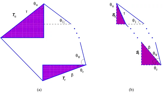
for anyK >0. The proof forE(Mn(Zr)) is similar. When|Iu|= 0, there are two further possible cases: P1⊂ P and P16⊂ P. Let τ denote the segment on P having the common intersection pointIuwiths1. In the first caseP1⊂ P, letTube the right triangle
with hypotenuseτ and letθu be the angle between the hypotenuse and the opposite; see Figure 4(a). In
the second case, we denote bySu andθu the right triangle with hypotenuseτ and the angle formed by
τ and the opposite, respectively; see Figure 4(b).
In a parallel manner, when|Ir|= 0, we distinguish between Pν ⊂ P andPν 6⊂ P and defineβ, Tr,Sr,
r u u (a) (b) ν ν T T S S θ β τ τ 000000000000 000000000000 000000000000 000000000000 000000000000 000000000000 000000000000 000000000000 000000000000 111111111111 111111111111 111111111111 111111111111 111111111111 111111111111 111111111111 111111111111 111111111111 000000000000 000000000000 000000000000 000000000000 000000000000 000000000000 000000000000 000000000000 000000000000 000000000000 000000000000 000000000000 000000000000 000000000000 000000000000 000000000000 000000000000 000000000000 000000000000 111111111111 111111111111 111111111111 111111111111 111111111111 111111111111 111111111111 111111111111 111111111111 111111111111 111111111111 111111111111 111111111111 111111111111 111111111111 111111111111 111111111111 111111111111 111111111111 β θ θ θ θ θ θ θ r r 1 u u 1 r
Figure 4: Illustration of the cases whenIu∩Ir=∅and either |Iu|= 0or |Ir|= 0.
Lemma 9. If|Iu|= 0 andP1⊂ P then
E(Mn(Tu)) = √ 1
cotθucotθ1+ 1 log
√
cotθucotθ1+ 1 + 1 √
cotθucotθ1+ 1−1
+O(n−1/2); (3.5)
if|Ir|= 0 andPν ⊂ P then
E(Mn(Tr)) = √ 1
cotθrtanθν+ 1
log √
cotθrtanθν+ 1 + 1
√
cotθrtanθν+ 1−1
+O(n−1/2). (3.6)
Proof.By (3.1),
E(Mn(Tu)) = n
|P|
Z ε
0
Z ytanθu 0
1− 1 |P|
xy−tan2θux2+cotθ1 2 y
2
n−1
dxdy+O(n−K),
for anyK > 0. The remaining proof of (3.5) is similar to the derivations for (3.4). The result (3.6) is
proved in a similar manner.
Lemma 10. If |Iu|= 0andP16⊂ P then E(Mn(Su)) =
tanθu
cotθ1−tanθu
+O(n−1/2); (3.7)
if|Ir|= 0 andPν 6⊂ P then
E(Mn(Sr)) = tanθr
cotθν−tanθr +O(n
−1/2). (3.8)
Proof.These follow from the integral representations
E(Mn(Su)) = n
|P|
Z ε
0
Z ytanθu 0
1−tan2 θ1
|P| (ycotθ1−x) 2n−1
dxdy+O(n−K),
E(Mn(Sr)) =
n |P|
Z ε
0
Z ytanθr 0
1−tan2 θν
|P| (ycotθν−x) 2n−1
and an analysis similar to the preceding cases.
When some part ofPj lies outsideP, namely,Pj∩ P 6=Pj, we have
E(Mn(P1∩ P)) = E(Mn(P1)−E(Mn(Su)),
E(Mn(Pν∩ P)) = E(Mn(Pν)−E(Mn(Sr)),
E(Mn(Pj∩ P)) = E(Mn(Pj)) +O(n−K) (j= 2, . . . , ν−1).
Let
D=P \(P1∪ · · · ∪ Pν∪ R1∪ · · · ∪ Rν−1∪(Zu orTu)∪(Zr orTr));
(see Figure 3). Then E(Mn(D)) = O(n−K), for any K > 0, since there exists an ε > 0 such that
|P ∩ {s : s≻t}|> ε, for allt∈ D. Thus whenIu∩Ir=∅, we have
E(Mn) = X
1≤j≤ν
E(Mn(Pj)) + X
1≤j≤ν−1
E(Mn(Rj)) + 1{|Iu|>0}E(Mn(Zu)) + 1{|Ir|>0}E(Mn(Zr)) + 1{|Iu|=0}1{P1⊂P}E(Mn(Tu)) + 1{|Ir|=0}1{Pν⊂P}E(Mn(Tr))
−1{|Iu|=0}1{P16⊂P}E(Mn(Su))−1{|Ir|=0}1{Pν6⊂P}E(Mn(Sr)) +O(ν+ 1)n−1/2.
This proves (1.3) whenπ1>0 with
π3 = −ν+
X
1≤j≤ν−1
p
tanθj+1 2p
tanθj+1−tanθj
log
p
tanθj+1+ptanθj+1−tanθj p
tanθj+1−ptanθj+1−tanθj
+ 1{|Iu|>0}
γ 2 +
1 2log
2|Iu|2tanθ1 |P|
1 + 1{|Ir|>0}
γ 2 +
1 2log
2|Ir|2cotθν
|P|
+ 1{|Iu|=0}1{P1⊂P}
1 √
cotθucotθ1+ 1 log
√
cotθucotθ1+ 1 + 1 √
cotθucotθ1+ 1−1 + 1{|Ir|=0}1{Pν⊂P}
1 √
cotθrtanθν+ 1
log √
cotθrtanθν+ 1 + 1
√
cotθrtanθν+ 1−1
−1{|Iu|=0}1{P16⊂P}
tanθu
cotθ1−tanθu −
1{|Ir|=0}1{Pν6⊂P}
tanθr
cotθν−tanθr
. (3.9)
Case 2: Iu∩Ir6=∅. We further divide into four cases. First, if|Iu|>0 and|Ir|>0 (see Figure 5(a)),
then
E(Mn) =
n |P|
Z |Iu|
0
Z |Ir|
0
1− xy |P|
n−1
dydx+J+O(n−K)
= logn+γ+ log|Iu| |Ir|
|P| +J+O(n
−1/2),
whereJ denotes the contribution of the part inP outside the rectangle formed by the two segmentsIu
and Ir. If we are in the case shown in Figure 5(a), then the expected number of maxima contributed
from the triangle to the left ofIu (with spanning angleθu) is given by
n |P|
Z ε
0
Z ε
xcotθu
1− 1 |P|
xy+|Iu|y−
x2 2 cotθu
n−1
Similarly, the contribution from other parts ofP and the “overshoot” are allO(n−1).
On the other hand, if|Iu| >0 and |Ir| = 0 with angleθu at the upper-right corner (see Figure 5(b)),
then by a similar argument
E(Mn) =
n |P|
Z |Iu|
0
Z xtanθu 0
1− 1 |P|
xy−y 2 2 cotθr
n−1
dydx+O(n−1/2)
= 1
2logn+ γ 2 +
1 2log
2|Iu|2tanθu
|P| +O(n
−1/2).
[image:21.612.124.475.141.292.2]r θu θ (a) I (b) θ I I θ I I (c) r I I θ θ (d) u u u r r r u u u r r I
Figure 5: Illustration of possible cases when Iu∩Ir6=∅.
Similarly, if|Ir|>0 and|Iu|= 0 with angleθr at the upper-right corner (see Figure 5(c)), then
E(Mn) =
1 2logn+
γ 2 +
1 2log
2|Ir|2tanθr
|P| +O(n
−1/2).
Finally, if|Iu|=|Ir|= 0 with anglesθu andθrindicated as in Figure 5(d), then
E(Mn) =
n |P|
Z ε
0
Z xcotθu
xtanθu
1− 1 |P|
xy−tan2θux2−tan2θry2
n−1
dy+O(n−K)
=
Z cotθr tanθu
dy
2y−tanθu−y2tanθr +O(n
−1/2) (3.10)
= 1
2√1 + tanθutanθr
log √
1 + tanθutanθr+ 1−tanθutanθr
√
1 + tanθutanθr−1 + tanθutanθr
+O(n−1/2). (3.11)
Collecting the above results, we have whenIu∩Ir6=∅
π3=
γ+ log|Iu||Ir|
|P| , if |Iu||Ir|>0;
γ 2 +
1 2log
2|Iu|2tanθu
|P| , if |Iu|>0,|Ir|= 0, γ
2 + 1 2log
2|Ir|2tanθr
|P| , if |Iu|= 0,|Ir|>0, 1
2√1 + tanθutanθr
log √
1 + tanθutanθr+ 1−tanθutanθr
√1 + tanθ
utanθr−1 + tanθutanθr
, if |Iu|=|Ir|= 0.
(3.12)
This completes the proof of (1.3).
3.2
Asymptotic normality
triangleT is scale invariant. Assume thatν ≥1. LetSn :=P \ ∪1≤j≤νPj. Then, by our discussions in
Section 3.1,E(Mn(Sn)) =O(ν+ logn). From this and the inequality X
1≤j≤ν
Mn(Pj)≤Mn = X
1≤j≤ν
Mn(Pj) +Mn(Sn),
it follows that (Mn−π1n1/2)/(σ1n1/4) andWn:=P1≤j≤ν[Mn(Pj)−(|Pj|πn/|P|)1/2]/(σ1n1/4) have the same limit distribution. Let Φn and Φ denote the distribution functions ofWn andN(0,1), respectively.
We show that|Φn(x)−Φ(x)| →0 for allx∈R.
To that purpose, assume first that allPj, 1≤j ≤ν, are all right triangles. Define Πn to be the set of all
ν-tuplesρ= (r1, . . . , rν) of nonnegative integersrj such thatr1+· · ·+rν≤n. Let Ωρ be the event that
there are exactlyrj points lying inPj, whereρ∈Πn. Then Φn(x) =Pρ∈ΠnP(Ωρ)Φn,ρ(x),where Φn,ρ is the conditional distribution function of Wn under Ωρ. Let Yj := Mn(Pj). Observe that, under Ωρ,
these Yj’s are independent and that the distribution ofYj under Ωρ is the same as that of the number
of maxima ofrj iid points taken uniformly at random fromPj. Let Ψn,ρ be the conditional distribution
function (under Ωρ) of
Zn,ρ:= P
1≤j≤ν(Yj−Eρ(Yj))
P
1≤j≤νVarρ(Yj) 1/2,
whereEρ(Yj) :=E(Yj|Ωρ) and Varρ(Yj) := Var(Yj|Ωρ). Define µj :=|Pj|/|P|and the subset Π′n⊂Πn
by
Π′
n:= n
ρ= (r1, . . . , rν)∈Πn : |rj−µjn| ≤(µjn)1/2lognfor allj= 1, . . . , ν o
. (3.13) By (2.3), we have, uniformly for allρ∈Π′
n,
sup
x∈R
|Ψn,ρ(x)−Φ(x)|=o(1).
Thus to prove (1.7), it suffices to show that
(i) the probability of the union of Ωρ,ρ∈Π′n, tends to 1;
(ii) uniformly for allρ∈Π′
n,P(|Wn−Zn,ρ|> ε|Ωρ)→0, for anyε >0.
¿From these, we obtain, by Slutzky’s theorem (suitably modified under our conditioning setting; see [15, p. 254]), that|Φn,ρ−Φ(x)| →0, uniformly forρ∈Π′n, wherex∈R. Thus
|Φn(x)−Φ(x)| ≤ P ∪ρ∈Πn\Π′nΩρ
+ X
ρ∈Π′n
P(Ωρ)|Φn,ρ(x)−Φ(x)|
→ 0.
The proof of (i) usesP(X1∈ Pj) =µj and Bernstein’s inequality for binomial distributions (see [15, p.
111]), giving
P ∪ρ∈Πn\Π′nΩρ
≤ X
1≤j≤ν
P|Yj−µjn|>(µjn)1/2logn
≤ 2µ−j1/2exp
− log
2 n
2(1−µj) + 2(µjn)−1/2logn
→ 0. By (3.3), (2.2), and (3.13)), we deduce that
X
1≤j≤ν
Eρ(Yj)−π1n1/2=o(n1/4),
X
1≤j≤ν
x
y
µP
T
T
T
T
T
4
2
1
s
3
1
[image:23.612.133.464.91.218.2]1
Figure 6: “Paper-folding” triangulation ofP1.
for allρ∈Π′
n. Thus (ii) follows.
This proves the asymptotic normality ofMn(P) when bothP1andPν are right triangles.
Now assume that P1 is not a right triangle (it is then an obtuse triangle). We split P1 into 2µ right triangles and an obtuse triangle in the following “paper-folding” way (see Figure 6). Denote bys1 the hypotenuse ofP1 and call the point opposite to the hypotenusex. Make a right triangle by connecting a vertical line from x to s1. Assume that the horizontal line intersects s1 at y. Draw a vertical line fromy to the opposite. This results in two right triangles and an obtuse triangle. Call the right triangle sharing the same hypotenuse with s1 T1. Repeating µ−1 times the same construction in the obtuse triangle yieldsµright trianglesTi alongs1. We takeµ=⌊clogn⌋, wherecis properly chosen so that the
expected number of points lying in the obtuse triangle is≤n1/5and that the expected number of points in each Ti is ≥ n1/5. This is achievable since the area of the obtuse triangle contracts exponentially.
We then argue similarly as above, noting that the main contribution to Mn(P1) comes from Ti. The
asymptotic normality ofMn(P1) follows as above. The case whenPν is not a right triangle is similar.
This completes the proof of (1.7).
3.3
Variance
LetM∗
n := (Mn−π1n1/2)/(σ1n1/4). For the proof of Theorem 1 whenπ1>0, it remains to show (1.6). But this is an easy consequence of the asymptotic normality ofMn and (2.9) withm= 2. For,
E(Mn−π1n1/2)4=O
X
1≤j≤ν
EMn(Pj)−(|Pj|πn/|P|)1/2 4
=Oν(n),
implying that supnE(Mn∗4) =O(1) and consequently,Mn∗2 is uniformly integrable. The result (1.6) now
follows from dominated convergence theorem and (1.7).
4
Maxima in regions bounded above by a nonincreasing curve
We consider in this sectionC of the form (1.1)
wheref(x) is a nonincreasing function in the unit interval. We may assume for convenience that
Z 1
0
f(x) dx= 1.
LetC2(a, b) denote the set of real functions whose second derivatives are continuous in (a, b), wherea < b. For convenience we also define
C2(a, b) ={f ∈C2(a, b) : 0<|f′(x)|<∞, a < x < b}. The classification of critical points into|f′(x)|= 0,|f′(x)|=∞orf′
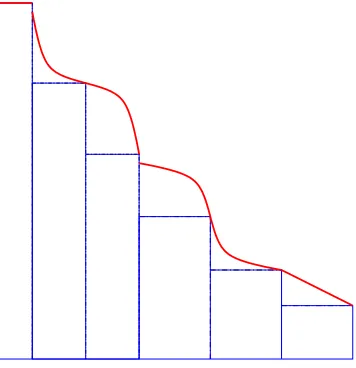
−(x)6=f+′(x) leads the study of the expected number of maxima to the following three prototypical cases of decreasingf (see Figure 7): (i) f ∈C2(0,1);
(ii) f(x) =η >0 for 0≤x≤ξ <1 andf ∈C2(ξ,1); or its symmetric (with respect to the liney =x) counterpart;
(iii) There is a unique critical pointξ∈(0,1) at whichf is continuous (to exclude jumps),f ∈C2(0, ξ) andf ∈C2(ξ,1).
(iii)
[image:24.612.132.460.336.394.2](i) (ii)
Figure 7: The three basic prototypes.
It is obvious that any piecewiseC2(0,1) decreasing functionsf can be finitely decomposed into the above prototypes and rectangles (see Figure 8). Our results provide a “transparent” connection between the coefficient of the logarithmic term and the local behavior off near each critical point. This connection, already observed by Devroye (1993), is made quantitatively more precise here. Note thatf may have critical points at the boundary (0 and 1) in the first case. Also ifξ= 1 in the second case, then Cis the unit square and the expected number of maxima is asymptotic to logn+O(1).
[image:24.612.210.388.505.689.2]Theorem 4. Assume thatf : [0,1]7→[0,∞)is nonincreasing,f(1) = 0 andR1
0 f(x) dx= 1. (i)If f ∈C2(0,1) and
f′(x) = −xα(a+o(1)), (4.1)
f′(1−x) = −xβ(b+o(1)), (4.2)
asx→0+, wherea, b >0,α >
−2 andβ >−1 (since f(x)≥0), then
E(Mn) = π0n1/2+ 1 3
α
α+ 2− β β+ 2
logn+o(logn).
(ii)If f(x) =η >0for 0≤x≤ξ <1,f ∈C2(ξ,1) and
f′(ξ+x) = −xα(a+o(1)), (4.3) f′(1−x) = −xβ(b+o(1)),
asx→0+, wherea, b >0 andα, β >−1, then E(Mn) =π0n1/2+
1 3
α+ 3
α+ 2− β β+ 2
logn+o(logn).
The symmetric version with respect to the liney=xhas the same asymptotic behavior.
(iii) Assume that ξ is the unique critical point in (0,1) at which f is continuous. If f ∈ C2(0, ξ),
f ∈C2(ξ,1),f satisfies (4.1) and (4.2), and
f′(ξ−x) = −xβ′(b′+o(1)), f′(ξ+x) = −xα′(a′+o(1)),
asx→0+, wherea′, b′ >0andα′, β′>−1, then
E(Mn) =π0n1/2+ 1 3
α
α+ 2 + α′
α′+ 2 −
β β+ 2−
β′
β′+ 2
logn+o(logn).
Thus the expected number of maxima,E(Rn), contributed from the rectangle, satisfies
E(Rn) = logn
α+ 2(1 +o(1)),
in case (ii) andE(Rn) =O(1) in the last case (see Figure 7). Under stronger conditions, our method of
proof can be further refined to make explicit theo-terms; see Bai et al. (2000).
Proof of Theorem 4. (Sketch) The starting point is the integral representation
E(Mn) = n Z 1
0
Z f(x)
0
1−
Z f−1(y) x
(f(t)−y) dt
!n−1 dydx
= n
Z 1
0 | f′(w)|
Z w
0
(1−A(x, w))n−1 dxdw, where|f′(w)|=−f′(w) for 0< w <1 andA(x, w) =Rw
w−x(f(t)−f(w)) dt. Take two small quantities
δ0=n−1/(α+2)(logn)2/(α+2) andδ1=n−1/(β+2)(logn)2/(β+2)and split the integral into three parts:
E(Mn) = n Z δ0
0 +
Z 1−δ1
δ0 +
Z 1
1−δ1
!
|f′(w)|Z
w
0
Then prove that
I1 =
(2πa)1/2 α+ 2 n
1/2δ(α+2)/2
0 +
α
3(α+ 2)logn+ α
3 logδ0+o(logn), I3 = (2πb)
1/2 β+ 2 n
1/2δ(β+2)/2
1 −
β
3(β+ 2)logn− β
3logδ1+o(logn), and that the main contribution toE(Mn) comes fromI2:
I2=π0n1/2−
(2πa)1/2 α+ 2 n
1/2δ(α+2)/2
0 −
(2πb)1/2 β+ 2 n
1/2δ(β+2)/2
1 +
β
3logδ1− α
3 logδ0+o(logn).
For details, see Bai et al. (2000).
Case (ii). (Sketch) It suffices to consider the contribution from the rectangleRn (see Figure 7) since
the other part is essentially covered by case (i). By (4.3),
E(Rn) = n Z ξ
0
Z η
0
1−(ξ−x)(η−y)−
Z f−1(y) ξ
(f(t)−y) dt
!n−1 dydx
∼ (α+ 1)
Z 1−ξ
0
w−1e−anwα+1/(α+2)−e−anξwα+1/(α+1)dw = logn
α+ 2+O(1).
The symmetric version ofE(Mn) with respect to the liney=xis similar.
5
Maxima in regions bounded by two increasing curves
The results in the preceding section give an interpretation of the “magic constant” 1/2 in the expansion (1.3). We give another different “structural interpretation” in this section by considering the region
C={(x, y) : 0≤x≤1,min{f(x), g(x)} ≤y≤max{f(x), g(x)}}, wheref(x) andg(x) are two nondecreasing function in the unit interval. Assume that
Z 1
0 |
f(x)−g(x)|dx= 1<∞, and that
f(1−x) = f(1)−xα(a+o(1)),
g(1−x) = f(1)−xβ(b+o(1)), (5.1)
asx→0+, wherea, b, α, β >0. We may assume thatf(x)
≥g(x) in the vicinity ofx= 1, namely,α > β ifα6=β anda < b ifα=β.
Theorem 5. Ifα > β≥0 then
E(Mn) = 1
β+ 1 − 1 α+ 1
where
c3 := logb β+ 1−
loga α+ 1+
β α(β+ 1)+
log(α+ 1) α+ 1 +
β(α+ 1)
α(β+ 1)log(β+ 1) − α
2+ 2α −β
α(α+ 1)(β+ 1)logα+ α−β
α(β+ 1)log(α−β);
on the other hand, if α=β then
E(Mn) =
1 α+ 1
Z b
a
dy
y−αa+1−bαy1/α1+1(α+1)/α
+o(1).
It is easily shown that
1 α+ 1
Z b
a
dy y− a
α+1 −
αy1+1/α
b1/α(α+1) ≥1,
meaning that there is at least one maximal point. Note that the expected number of maxima remains bounded for functions such asf(x) = 101
99x
1/100 andg(x) = 101 99x
100.
Proof of Theorem 5. (Sketch) Takeδ=δn=n−1/(α+1)(logn)2/(α+1).ThenE(Mn) =I1+I2, where
I1 = n
Z 1
1−δ Z f(x)
g(x)
(1−A(1−x,1−y))n−1dydx,
I2 = n
Z 1−δ
0
Z max{f(x),g(x)}
min{f(x),g(x)}
(1−A(1−x,1−y))n−1 dydx.
HereA(1−x,1−y) denotes the area of the region
{(u, v) : x≤u≤1;y ≤v≤f(1),min{f(x), g(x)} ≤v≤max{f(x), g(x)}}. By (5.1),
A(x, y) =xy−aα++ 1o(1)xα+1−(ββ+ 1)+o(1)b1/βy
1+1/β, (5.3)
uniformly for 0≤x≤δandφ(x)≤y≤γ(x).
Since for fixedxthe function A(1−x,1−y) is a nondecreasing function of y,
I2=O
n max
φ(δ)≤y≤γ(δ)e
−nA(δ,y)
=One−c4(logn)2=o(1).
Ifα=β, then by (5.3),
I1 ∼ n
Z δ
0
Z b
a
xαe−nA(x,xαy)dydx
∼ n
Z b
a Z ∞
0
xαexp
−nxα+1
y−α+ 1a − αy 1+1/α
(α+ 1)b1/α
dxdy
∼ α+ 11
Z b
a
dy y− a
α+1 −
αy1+1/α
On the other hand, ifα > β, then
I1 = n
Z δ
0
Z bxβ−α
a
e−nA(x,xαy)dydx+o(1)
= n
Z (b/a)1/(α−β)
0
Z bxβ−α
a
xαexp
−nxα+1
y− a α+ 1+
βb−1/β
β+ 1 x
−1+α/βy1+1/βdydx+o(1),
¿From this integral representation, the expansion (5.2) is obtained by using Mellin transform techniques.
See Bai et al. (2000) for details.
Remark. Ifβ = 0 thenE(Mn)∼α(logn)/(α+1); if, furthermore,f is linear, thenα= 1 which implies
that E(Mn)∼(1/2) logn. This essentially corresponds to the case |Iu|= 0 and |Ir|>0 in Section 3.1.
The case when α = ∞ and g is linear is similar. When both f and g are linear functions, we have α=β = 1, and thus
E(Mn(C)) = Z b
a
dy
2y−a−y2/b+o(1) = √
b 2√a+blog
p
b(b+a) +b−a
p
b(b+a)−b+a+o(1); which is essentially the case when|Iu|=|Ir|= 0; see (3.11).
6
Maxima in regions bounded above by an increasing curve
We prove Theorem 2 on Poisson approximations in this section.
6.1
Probability generating function
Let
Sm(u) =u(u+ 1)· · ·(u+m−1)
m! (m≥1)
denote the probability generating function of the number of maxima when the underlying regionC is a rectangle.
Proposition 2. LetF(x) =Rx
0 f(t) dt. Then for any nondecreasing function f E(uMn) = 1 + (u
−1) X 1≤j≤n
Sj−1(u)
n j
Z 1 0
F(x)n−jf(x)j(1−x)j−1dx (n≥1). (6.1)
Proof. We use a method similar to the proof of (2.4). Let V ={(xj, yj) : 1 ≤j ≤ n} be n iid points
chosen uniformly inC.
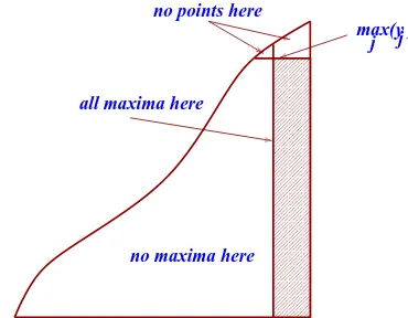
We first locate the pointp= (x, y) for whichy= max1≤j≤nyj. Then the number of maxima equals one
plus those in the (shaded) rectangle (see Figure 9). The probability that there are exactlyk points inV lying in the rectangle formed by (x, y) and (1,0) is equal to
pn,k(x, y) :=
n−1 k
Z f−1(y)
0
f(t) dt+y x−f−1(y) !n−1−k
00000 00000 00000 11111 11111 11111 0000000 0000000 1111111 1111111 00000 00000 11111 11111 0000 0000 0000 0000 0000 0000 0000 0000 0000 0000 0000 0000 0000 0000 0000 0000 0000 0000 1111 1111 1111 1111 1111 1111 1111 1111 1111 1111 1111 1111 1111 1111 1111 1111 1111 1111 00000000000 00000000000 11111111111 11111111111
no maxima here all maxima here
no points here
[image:29.612.200.385.90.234.2]max(y ) j j
Figure 9: Division ofC at the point withmax1≤i≤nyi; all other maxima are inside (and on) the rectangle.
Thus we have
E(uMn) = nu X 0≤k≤n−1
Sk(u) Z
C
pn,k(x, y) dxdy
= u X
0≤k≤n−1
pn,kSk(u),
where
pn,k =
n! k!(n−1−k)!
Z 1
0
Z f(x)
0
Z f�