AN IMPROVED VARIATIONAL METHOD FOR HYPERSPECTRAL IMAGE
PANSHARPENING WITH THE CONSTRAINT OF SPECTRAL DIFFERENCE
MINIMIZATION
Zehua Huang a, Qi Chen a, b , Yonglin Shen a, Qihao Chen a, Xiuguo Liu a
a Faculty of Information Engineering, China University of Geoscience, Wuhan, China- [email protected], (daoqiqi, yonglinshen)@gmail.com, [email protected], [email protected]
b Center for Spatial Information Science, The University of Tokyo, Tokyo, Japan
KEY WORDS: Image fusion, Pansharpening, Hyperspectral image, Variational model, Spectral fidelity, Spectral difference minimization
ABSTRACT:
Variational pansharpening can enhance the spatial resolution of a hyperspectral (HS) image using a high-resolution panchromatic (PAN) image. However, this technology may lead to spectral distortion that obviously affect the accuracy of data analysis. In this article, we propose an improved variational method for HS image pansharpening with the constraint of spectral difference minimization. We extend the energy function of the classic variational pansharpening method by adding a new spectral fidelity term. This fidelity term is designed following the definition of spectral angle mapper, which means that for every pixel, the spectral difference value of any two bands in the HS image is in equal proportion to that of the two corresponding bands in the pansharpened image. Gradient descent method is adopted to find the optimal solution of the modified energy function, and the pansharpened image can be reconstructed. Experimental results demonstrate that the constraint of spectral difference minimization is able to preserve the original spectral information well in HS images, and reduce the spectral distortion effectively. Compared to original variational method, our method performs better in both visual and quantitative evaluation, and achieves a good trade-off between spatial and spectral information.
1. INTRODUCTION
Hyperspectral (HS) technology plays an important role in numerous scientific domains, including geological survey (Van der Meer et al., 2012), material identification (Li et al., 2012), and remote sensing (Adam et al., 2010). HS images can acquire abundant spectral information with a continuous and fine-grained spectral coverage in multiple bands, which results in the widespread use of HS remote sensing in many applications, such as surface mineralogical mapping (Van der Meero & Bakker, 1997), water quality monitoring (Brando & Dekker, 2003), and detection of crop disease (Grisham et al., 2010). However, owing to the limited amount of incident energy of HS images, critical trade-offs must be made between spatial and spectral resolutions in the design of optical remote sensing systems (Loncan et al., 2015). Thus, the spatial resolution of the HS image is generally lower than that of other remote sensing images, making it more difficult to recognize visual features, especially those composed of plural pixels, such as the edge and shape of ground objects (Yokoya et al., 2012). To overcome this problem, the technique of image pansharpening integrates HS image with panchromatic (PAN) image, which has high spatial resolution but only with a single spectral band. By combining the spectral information in HS images and spatial information in PAN images, image pansharpening aims at generating an ideal image with high spectral and spatial resolutions. With its detailed spatial information and fine-grained spectral information, the pansharpened image can be used in applications requiring more accurate object recognition and classification, such as in geology and mineral identification, agriculture statistics, and analysis of urban surface (Segl et al., 2003).
In the pansharpening process of HS images, spectral distortion of the image is an important potential problem. If pansharpened images with distorted spectral information are employed in applications such as geological phenomenon identification, then the accuracy of data analysis will be directly affected, and the effectiveness of the pansharpened images will be significantly reduced. Therefore, to reduce spectral distortion in the pansharpening process, a preferred pansharpening algorithm should both improve the spatial resolution of the HS image and minimize the spectral difference between the images before and after the process.
Current pansharpening methods broadly fall into three major groups according to their underlying principles (Vivone et al., 2014) :
(1) Component Substitution (CS). CS is performed by transforming the HS image into the frequency domain. With this method, the image is first divided into spatial and spectral information, then the original spatial information component is substituted with a PAN image. Inversely transforming the components generates the pansharpened image. Numerous algorithms, including intensity-hue-saturation transform (Tu et al., 2001), principal component analysis (PCA) (Chavez et al., 1989), and Gram-Schmidt (GS) pansharpening (Laben & Brower, 2000), can be classified as CS approaches. These algorithms generally achieve good spatial information fidelity and are easy to implement (Tu et al., 2001). However, considering that the different wavelength ranges of the HS and the PAN images may lead to large radiation offset during the component substitution, severe spectral distortion may result from CS approaches (Thomas et al., 2008).
(2) Multi-resolution Analysis (MRA). In these approaches, the spatial information of the PAN image is extracted based on MRA, and the spatial details of the hyperspectral image can be enhanced using the extracted spatial information. MRA approaches contain algorithms such as decimated wavelet transform (Mallat, 1989), undecimated wavelet transform (Loncan et al., 2015) and Laplacian pyramid (Aiazzi et al., 2006). These algorithms perform well in terms of temporal coherence and robustness (Segl et al., 2003), but blurred edge, texture, and shifted pixels may exist in the pansharpened image (Alparone et al., 2007). Improvements are still needed to avoid aliasing and spatial detail distortion.
(3) Bayesian Approaches. These approaches perform image pansharpening by first determining the prior probability distribution of the image sampling area, and then designing statistical measurements in a Bayesian framework (Zhang et al., 2009). Various statistical models based on the Bayesian theory have been proposed, such as subspace-based regularization fusion (Simoes et al., 2015), sparse-representation-based fusion (Wei et al., 2015), and variational approach (Ballester et al., 2003). Among them, the variational approach is one of the widely-applied pansharpening methods, which mainly includes the wavelet variational pansharpening (Moeller et al., 2009), similarity-based variational pansharpening (Shi et al., 2011), and fast variational pansharpening (Zhou et al., 2012). In a typical variational approach, an energy function is constructed based on two principles: one describes the spatial similarity between the HS image and the PAN image, and the other is the linear relationship between corresponding bands of the HS image and the pansharpened image. The pansharpened image can be reconstructed by seeking the optimal solution of the energy function. As a fusion method at pixel level, variational pansharpening can preserve the original spectral feature by enhancing the spectral correlation (Moeller et al., 2009). Meanwhile, the fidelity of spatial and spectral information can be well balanced in the pansharpened results.
Although most of the abovementioned approaches can enhance the spatial detailed information of the HS image, severe spectral distortion may still occur during the pansharpening process. Compared with other methods, the advantage of variational pansharpening lies in achieving a good trade-off between spatial information and spectral information. However, the classical variational method remains likely to generate obvious distortion of spectral curves and pixel errors when processing HS images. To further reduce the spectral distortion and error, in this paper we propose an improved variational method for HS image pansharpening with the constraint of spectral difference minimization. First, assuming that the spatial information of the PAN image and the pansharpened image are highly similar, a spatial fidelity term is defined using the second derivative and space vector field of images. Then, to minimize the spectral difference between the HS and the pansharpened image, a spectral fidelity term is defined using the spectral difference value and spectral vector field of images. Combining these two fidelity terms to construct an energy function can generate the pansharpened image by finding the optimal solution using the gradient descent method.
Two sets of HS images from the satellites Huanjing-1A (HJ-1A) and Earth Observing-1 (EO-1) are used for the pansharpening experiment. The experimental results indicate that the pansharpened images generated by our method have relatively high visual quality and clear details of ground objects. In particular, the spectral fidelity of the methods is also evaluated by the spectral angle mapper and the spectral correlation coefficient indexes. They illustrated that our method out-performs the fusion approaches from the literature. Aside from
this, the statistical analysis of multiple indexes proves that our method has advantages over the original variational pansharpening. The improvements are achieved in both spatial and spectral information fidelity.
The remainder of the paper is organized as follows. In Section II, we introduce the original variational framework. Section III provides a detailed description of the improved method. In Section IV, the experimental results and evaluation are presented, including the comparison between the experimental methods. Conclusions are drawn in Section V.
2. THE ORIGINAL VARIATIONAL PANSHARPENING
In this section, we firstly review the original variational pansharpening method proposed by Ballester (Ballester et al., 2003). The original variational pansharpening fuses images by constructing the energy function based on the hypotheses of the spatial similarity, the image relation and the convolution filtering expression.
The spatial similarity assumes that the geometry of the spectral channels at high resolution follows the geometry of the panchromatic image. According to the mathematical morphology, the geometric information and spatial information of an image are mainly contained in the level sets (Ballester et al., 2003). The level sets can be expressed by the vector field defined in (Ballester et al., 2003). Since the abundant spatial information contained in PAN image should be also contained in pansharpened image, it is assumed that each band of the pansharpened image aligns with the normal vector field of the PAN image (Ballester et al., 2003). Then, the following relationship is derived:
, 0
*
ui ui (1)
where
u
i represents the ith band of the pansharpened image u, denotes the normal vector field of the PAN image, thegradient field 2 2 2
) / ( ) /
(
ui ui x ui y . ui /xand
y ui
/ represent the partial derivative of fused image in the x and y directions. Every band of the fused image should satisfy (1). Thus, the spatial fidelity term of the variational model is constructed:
, ) * (
1
n i
i i
g u u
E (2)
where n is the number of bands. R2 denotes an open, bounded domain with a Lipschitz boundary.
Image relation hypothesis proposed that the PAN image corresponds to the weighted sum of each multispectral image. The weights represent the energies of different spectral bands. Based on the relation, the second term can be derived:
,
)
( 2
1
u P
E n
i i i
r (3)
where 1...n are the weighting coefficients of each channel, P denotes the PAN image.
The convolution filtering assumption expressed that the low resolution image is formed from the high resolution image by the low-pass filtering and the down-sampling. This constraint is used to write the third term as
*
,1
2
n i
i i i s
f k u H dx
E (4)
where s is a Dirac’s comb defined by the grid S,
k
iis the convolution kernel of the low-pass filter, Hi represents the ith channel of the original HS image H.
pansharpened image. Thus, the best quality pansharpened image can be generated based on the solution of the functional minimization. To find the solution, the gradient descent method is applied to derive the iteration scheme. Then, the result image is constructed.3. THE IMPROVED VARIATIONAL
PANSHARPENING
The original variational pansharpening method may lead to the spectral distortion when enhancing the spatial information in the hyperspectral image. To preserve the precise spectral information, our main contributions are designing a spectral fidelity term and constructing the improved energy function.
3.1 The Improved Variational Function
We assume that the spectral information of the pansharpened data should be close to that of the HS data. Thus, the pansharpened images keep the spectral characters of the HS images. To quantitatively analyze the characters of the spectrum, the spectral difference is used in our approach. This measurement represents the difference between the target band and its adjacent band in the image. The spectral difference is The spectral differences make up the spectral vector field which could accurately describe the change direction of the spectrum. In our approach, the spectral vector field is defined as
,
Since the spectral information of the original HS image and the pansharpened image should be highly similar, we assume that the spectral differences of HS image are linear approximate to those of pansharpened image:
, spectral differences of the pansharpened image, is proposed in our approach, which aims at match the original spectral differences with the pansharpened image. It can be obtained by
. Since the spectral difference of each channel is computed refer to the previous channel, the first channel of the two images are used as the reference in our approach. After the spectral difference multiplying by, we derive (10) from (8):
. the spectral information is constructed in our approach as
.
During the processing, if the value of the spectral fidelity term is close to 0, it indicates high similarity between the spectral information of the resulting image and the original HS image. Thus, high spectral quality is achieved.
Our improved variational pansharpening function is constructed by adding the proposed spectral fidelity term and the original spatial fidelity term. The mathematical representation is
.
s
g E
E
E (12)
The detailed description of the energy function in our method is achieved: corresponding information in the pansharpened image and the original image. the optimal solution of this function can be used to generate the pansharpened image.
3.2 Optimum Parameter Computation and Numerical Method
A variety of methods can be used to find the optimal solution of the variational model. In this study, the widely used gradient descent is chosen as our approach. This method creates an iterative function and searches the minimum value along the gradient descent direction. When the function reaches the local minimum value, we produce the final high-quality pan-sharpening image and terminate the process. First, we express the iterative function of our energy function in mathematical form.
The first-order differential form of energy equation (13) can be expressed as
definition of gradient, the arbitrary band is
.
Therefore, the iterative function of the gradient descent method is as follows:
3.3 Procedures
From the above discussion, the improved variational method is presented in
The workflow of our method can be demonstrated as follows: 1) The HS image and PAN image are preprocessed. Then,
the original HS image is oversampled to the resolution of the PAN image. The oversampled HS image and PAN image refer to the initial input images. The spectral differences and spectral level sets of the original HS image are computed.
2) The spatial fidelity term is computed by using the derivative of the PAN image and each band in the pansharpened image uk-1. The term is used to enhance the spatial information of the pansharpened image uk in the kth iteration.
3) The spectral differences of pansharpened image uk and original HS image are obtained based on the definition. Meanwhile, the spectral vector field Duand the coefficient
k
are computed. Then, we constructed the spectral fidelity term, which helps to correct the value of spectral information in uk.
4) The iterative process is constructed using the spatial fidelity term and the spectral fidelity term of pansharpened image. After that, the corrected image can be obtained.
5) After the new pansharpened image uk is generated by the function, we return to step (2) to reconstruct a new iteration using uk . The process continues until the number of iterations k meets the requirements.
4. EXPERIMENTS AND DISCUSSION
4.1 Dataset
Two sets of HS images obtained by the HJ-1A and EO-1 satellites are used in our experiment. Every dataset consists of a scene of a low-resolution HS image and a scene of a high resolution PAN image. The first dataset is of the Zijin Mountain mining area, in Fujian Province, China, with vegetation covers and exposed rocks. The second dataset is of Shanghai, an eastern city of China, where the main terrain is urban and partly fluvial. With these datasets, the performance of our methods in natural and urban terrains can be evaluated comprehensively. Detailed information of the datasets is presented in Table 1.
4.2 Evaluation Indexes
As a reference image is generally not available, we adopt the commonly used evaluation method in the pansharpening area to avoid this problem (Loncan et al., 2015). First, the spatial quality is evaluated by comparing the PAN image with each band of the fused image using an appropriate criterion. Then, the fused image is spatially degraded to a lower resolution of the original HS image. Afterward, these two images are compared to assess the extent of modification of the spectral information by the fusion method.
Both visual and quantitative evaluations are carried out in this paper. Four indexes are selected in our experiments (Loncan et al., 2015):
1) Spectral angle mapper. SAM is an important index that can evaluate spectral distortion quantitatively. The ideal value is 0.
2) Relative dimensionless global error in synthesis. ERGAS, as a global spectral quality index, considers the root mean square error of each band. The ideal value is 0.
3) Correlation coefficient. CC can represent the correlation degree between the pansharpened image and the reference image. The ideal value is 1.
4) Average gradient. AG describes the changing feature of image texture and the detailed information. Larger values of the average gradient correspond to more spatial details (Shi et al., 2011).
4.3 Results and Comparison
Comparative experiments were conducted with six widely used pansharpening methods including PCA (Chavez et al., 1989), smoothing filter-based intensity modulation (SFIM) (Liu, 2000), GS pansharpening (Laben & Brower, 2000), modulation transfer function with generalized Laplacian Pyramid (MTF_GLP) (Aiazzi et al., 2006), coupled nonnegative matrix factorization unmixing fusion (CNMF) (Yokoya et al., 2012), and original variational pansharpening (Ballester et al., 2003). The toolbox containing MATLAB implementations of all of the aforementioned methods can be downloaded online (Loncan, 2015b).
The same band images are selected from the results of two datasets, and shown in Figures 1, and 2, respectively. Tables 2 and 3 show the evaluation indexes of the two datasets. Each dataset is processed through all the methods mentioned above. The best two methods are highlighted in these tables. As demonstrated by the results, PCA and GS can only enhance spatial details, and they generate severe spectral distortion. SFIM and original variational pansharpening may produce blurring and aliasing effects on pansharpened images. Furthermore, CNMF and MTF_GLP perform ordinarily in quantitative evaluation. Clearly, each method has a problem either in spatial fidelity or in spectral fidelity. On the other hand, the images pansharpened by our method have abundant spatial information as well as good performance in spectral quantitative evaluation. A detailed discussion follows.
4.4 Discussion
An improved variational method for HS image pansharpening is proposed in this paper. The main features of the proposed method are the use of spectral difference and the construction of the spectral fidelity term in the improved variational model, which can correct the spectral distortion in pansharpened images. The performance or accuracy of the proposed method can be assessed from the following aspects:
Dataset ID Dimensions Spatial
resolution Bands Satellite
Longitude /ºE
Latitude /ºN
1 PAN 400*400 HS 60*60
15m 100m
1 115
Landsat-8 HJ-1A
116.37- 116.43
25.16- 25.21
2 PAN 480*480 HS 160*160
10m 30m
1 150
EO-1 EO-1
121.54- 121.57
31.36- 31.39
4.4.1 Spatial Information Fidelity
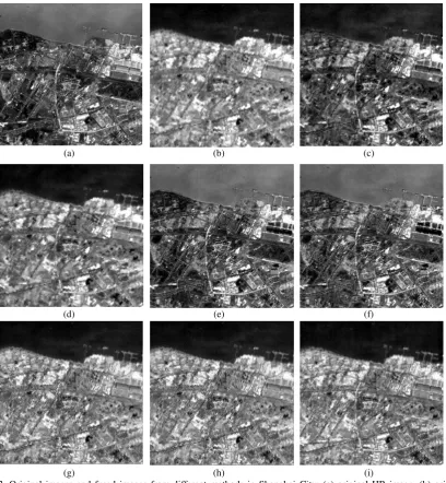
Improved variational pansharpening, as a pixel-level fusion method, can correct errors for each pixel. Unlike feature-level fusion in other related studies, our method directly utilizes a PAN image without transformation or multi-resolution analysis, thereby preserving more of the original details. CNMF, a representative of feature-level fusion, and the error of its reconstructed images may be influenced by the accuracy of unmixing (Yokoya et al., 2012). Figure 2 shows that the buildings are clear in (c) but a little blurry in (i). The results generated by our method are more similar to the PAN image.
During the spatial information injection process, the spatial vector field applied in this study is found to be more suitable than other methods. This strategy extracts details by using the image gradient in the x and y directions. This image gradient records the changes between adjacent pixels. Thus, the spatial information extracted has a close relationship with the global image. As proven in many experiments, the detailed spatial information can be well preserved in this manner, resulting in greatly improved spatial quality (Ballester et al., 2003, Moeller et al., 2009). By contrast, MTF_GLP utilizes the ratio of PAN image to low-pass filtered image to enhance fusion image spatial details (Aiazzi et al., 2006), which may easily give rise to blurring edges. This effect is proven in Figure 2(h). A large
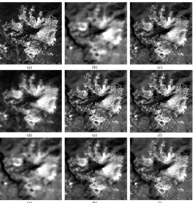
(a) (b) (c)
(d) (e) (f)
(g) (h) (i)
Figure 1. Original images and fused images from different methods in Zijin Mountain Mining Area: (a) original HR image, (b) original HS image, (c) proposed method, (d) original variational method, (e) PCA, (f) GS, (g) SFIM, (h) MTF-GLP, (i) CNMF.
Method SAM ERGAS Spectral CC Spatial CC AG
proposed method 0.0520 1.8742 0.8942 0.8817 1.0007
original method 3.1590 5.9591 0.8657 0.8808 0.8911
PCA 2.2345 3.0237 0.7868 0.8940 1.2529
GS 2.2824 3.0826 0.7766 0.9018 1.2547
SFIM 0.8004 1.3769 0.9556 0.7468 1.1865
MTF_GLP 1.4646 2.2683 0.8863 0.8267 1.4477
CNMF 2.6630 2.3412 0.8359 0.8860 1.0353
number of ground objects are difficult to identify, but (c) generated by our method is clear. Moreover, as shown by the indexes in Table 2, the spatial correlation coefficient of MTF_GLP is 0.8267, which performs worse than 0.8817, which achieved by our method.
In our energy function, the spectral gradient we use to preserve spectral information does not obviously impair the spatial information quality. By contrast, the smoothing filter used in SFIM may reduce the spatial quality by blurring the object edges. In Figure 1, for example, image (c) shows good performance, while Figure 1(g) generated by SFIM is
excessively smoothed and shows degraded mining area. In quantitative evaluation, the spatial correlation coefficient is 0.7468 in Table 2, our method is superior to this index. Compared with the original variational methods, the proposed method increases the spatial correlation coefficient from 0.8808 to 0.8817 in Table 2, and average gradient also increases from 0.8911 to 1.0007. These results demonstrated that our method performs better than most of the methods excepting PCA and GS. The quantitative evaluation and spatial details are both improved. Meanwhile, the dispersion statistics proved our method also has better stability during the experiments.
(a) (b) (c)
(d) (e) (f)
(g) (h) (i)
Figure 2. Original images and fused images from different methods in Shanghai City: (a) original HR image, (b) original HS image, (c) proposed method, (d) original variational method, (e) PCA, (f) GS, (g) SFIM, (h) MTF-GLP, (i) CNMF.
Method SAM ERGAS Spectral CC Spatial CC AG
proposed method 0.055 2.6882 0.8954 0.5566 0.1556
original method 7.1600 43.6790 0.8652 0.5838 0.1196
PCA 13.7080 19.6252 0.4006 0.9343 0.2367
GS 11.1873 18.2382 0.4229 0.9264 0.2351
SFIM 2.0633 28.3020 0.8466 0.3635 0.2830
MTF_GLP 2.2095 8.1352 0.8927 0.5130 0.2608
CNMF 2.0502 5.3051 0.9251 0.4295 0.1609
4.4.2 Spectral Information Fidelity
As spectral information and spatial information affect each other, a trade-off between them is of great significance in pansharpening. By finding the global minimization of the energy function, our method can balance different information to obtain the optimal overall quality. In the comparison, PCA and GS give priority to spatial information when substituting the components. Thus, the mean values of spectral correlation coefficients and SAM of PCA are 0.7868 and 2.2345 respectively, and 0.7766 and 2.2824 for GS. The indexes indicate that these two methods readily produce large spectral distortion. HowevEr, our method achieves much less spectral distortion than PCA and GS. As shown in Table 2, the spectral correlation coefficients and SAM of our method are 0.8942 and 0.052 respectively, both ranking first among the seven methods. In our experiments, the good performances of spectral quality prove the superiority of the spectral fidelity term in our variational method. Gradually correcting the difference between adjacent bands could accurately preserves the original spectrum. In other methods, CNMF obtains the endmember spectra by matrix factorization, which may lead to a small distortion. The fidelity terms of original variational pansharpening could not correct the distorted spectral information accurately. As shown in Table V, the ERGAS and SAM of CNMF are 3.1121 and 2.4057, while original variational pansharpening achieve 17.4987 and 4.0511; our results are thus better. The spectral correlation coefficient of our method and the original variation method are very close.
More details of spectral curves can be achieved by using the spectral difference. This outcome can be proved by the high similarity between the spectral curves generated by our method and the original curves. In comparison, MTF-GLP uses Laplacian pyramid to analyze the original HS images; this strategy does not meet the requirements of spectral accuracy. Additionally, the ERGAS and SAM of MTF_GLP are 4.0787 and 1.5873. Thus, these two indexes rank behind ours.
Compared with the original variational method, the values in Table 2 show that the improved method reduces SAM from 3.1590 to 0.0520, the ERGAS decreases from 5.9591 to 1.8742, the spectral correlation coefficients have close performance. Clearly, the proposed method improves the spectral quality evaluation indexes obviously, and protects the spectral information better than most other methods.
4.4.3 Overall Evaluation
The previous discussion indicates that the PCA and GS methods preserve spatial information best but produce serious spectrum distortion. SFIM performs well in all indexes, but blurred edges in the resulting image make practical interpretation difficult. CNMF has average performance in the quantitative evaluation. Moreover, MTF_GLP and the original variational pan-sharpening produce the aliasing phenomenon, which results in the lower image visual quality. Compared with the poor performance achieved by these methods, the proposed method used in the dataset is proven to be better. Its advantages are as follows:
(1) The proposed method can produce high-quality images with clear object edges. The spatial correlation coefficient and average gradient in Table 2 are 0.8817 and 1.0007, which indicate that its spatial information quality is obviously improved.
(2) The spectral information of the pansharpened image is most similar to the original HS image. The indexes SAM and ERGAS are the best among the methods, and the spectral correlation coefficient in Table 2 is 0.8942, which ranks in the top three.
(3) Our method not only achieves good performance in terms of spectral fidelity, but it also enhances the spatial information. In general, our method could achieve pansharpening images with better overall quality than the PCA, GS, MTF_GLP, CNMF, and SFIM methods. Particularly, when compared with the original variational pansharpening, the improved method strengthens the low spatial resolution image while preserving the spectral property very well.
4.4.4 Sensitivity Analysis of Parameters
The number of iterations k, step size ∆t, and the weighting
factors γ, η are the key parameters defined in our approach.
These parameters are determined according to their influence on the quality of the results. Sensitivity analysis is conducted according to the results for dataset 1and expanded to other datasets.
Parameter k is used to determine the number of iterations; when this parameter increases from 1, the result of our function is gradually optimized. The step size determines the correction value for each iteration. A small step size could correct small distortions to further improve the image quality. Comprehen-sively considering the image quality and computational quality and computational amount, we set the iteration number to 8 and the step size to 0.1.
After the step size and iteration numbers were determined, we
discussed the weighting factors. γ and η are used to maintain a
balance between spatial fidelity and spectral fidelity. The influence of these two parameters can generally be concluded as follows: when γ increases, the spatial information in the
pansharpened images are enhanced; as η increase, the spectral
information is increasingly preserved. Our method obtains a
better global quality if γ=0.2 and η=10. Thus, these are the most reasonable weighting factors.
5. CONCLUSION
Obvious distortion of spectral information exists among images pansharpened by commonly used methods. To resolve this issue, an improved variational method for HS image pansharpening with the constraint of spectral difference is proposed. First, the constraints of spectral difference and the spatial information similarity between pansharpened images and PAN images are combined to construct the energy function. Subsequently, the pansharpened image is generated by finding the optimal solution through gradient descent method. The main contribution of this study is the adoption of the new constraint of spectral difference minimization in the variational model. This constraint uses the difference between adjacent bands of images to correct spectral distortion.
Two sets of HS images from the satellites HJ-1A and EO-1 are used to evaluate the performance of the proposed approach. Meanwhile, six commonly used methods including the original variational pansharpening, PCA, GS, SFIM, MTF-GLP, and CNMF are applied as contrasts. The results achieved by our method demonstrate that the spatial correlation coefficient and average gradient are 0.8817 and 1.0007 respectively, which are higher than those of many other methods. These results indicate that our method can preserve details of the PAN image well. In the evaluation of spectral quality, given that the SAM, the spectral correlation coefficient and the ERGAS are 0.0520, 0.8942 and 1.8742, respectively, which rank in the top two. In conclusion, these findings suggest that, compared to other methods, our method can achieve better performances in both spatial and spectral fidelity.
may be enhanced by the spectral fidelity processing, which may lead to the lower global quality of results. In addition, automatic parameter selection is not currently considered in our function. An adaptive weighting function iteration algorithm can process massive amounts of data efficiently because the parameter analysis can be omitted. These problems will be considered in our future studies.
ACKNOWLEDGEMENTS
This research was supported by the China Postdoctoral Science Foundation with Project Number 2016M590730 and the National Natural Science Foundation of China with Project Number 41471355 and 41601506.
REFERENCES
Adam E., Mutanga O., Rugege D., 2010. Multispectral and hyperspectral remote sensing for identification and mapping of wetland vegetation: a review. Wetlands Ecol. and Manag. 18(3), pp. 281-296.
Aiazzi B., Alparone L., Baronti S., Garzelli A., Selva M., 2006. MTF-tailored multiscale fusion of high-resolution MS and Pan imagery. Photogramm. Eng. Remote Sens. 72(5), pp. 591-596.
Alparone L., Wald L., Chanussot J., Thomas C., Gamba P., Bruce L. M., 2007. Comparison of pansharpening algorithms: Outcome of the 2006 GRS-S data-fusion contest. IEEE Trans. Geosci. Remote Sens. 45(10), pp. 3012-3021.
Ballester C., Caselles V., Igual L., Verdera J., Roug B., 2006. A variational model for P+ XS image fusion. Int. J. Comput. Vision 69(1), pp. 43-58.
Brando V. E., Dekker A. G., 2003. Satellite hyperspectral remote sensing for estimating estuarine and coastal water quality. IEEE Trans. Geosci. Remote Sens. 41(6), pp. 1378-1387.
Chavez P. S. Kwarteng A. Y, 1989. Extracting spectral contrast in Landsat Thematic Mapper image data using selective principal component analysis. Photogramm. Eng. Remote Sens. 55, pp. 339-348.
Grisham M. P., Johnson R. M., Zimba P. V., 2010. Detecting Sugarcane yellow leaf virus infection in asymptomatic leaves with hyperspectral remote sensing and associated leaf pigment changes. J. Virol. Methods 167(2), pp. 140-145.
Laben C. A., Brower B. V., 2000. Process for enhancing the spatial resolution of multispectral imagery using pan-sharpening: U.S. Patent 6,011,875.
Li F., Ng M. K., Plemmons R. J., 2012. Coupled segmentation and denoising/deblurring models for hyperspectral material identification. Numer. Linear Algebra Appl. 19(1), pp. 153-173.
Liu J. G., 2000. Smoothing filter-based intensity modulation: A spectral preserve image fusion technique for improving spatial details. Int. J. Remote Sens. 21(18), pp. 3461-3472.
Loncan L., De Almeida L. B., Bioucas-Dias J. M., et al., 2015. Hyperspectral pansharpening: A review. IEEE Geosci. Remote Sens. Mag. 3(3), pp. 27-46.
Loncan L., 2015b. Available online: http://openremotesensing. net/index.php/codes/.
Mallat S G., 1989. A theory for multiresolution signal decomposition: the wavelet representation. IEEE Trans. Pattern Anal. Machine Intell. 11(7), pp. 674-693.
Moeller M., Wittman T., Bertozzi A. L., 2009. A variational approach to hyperspectral image fusion. Proc. SPIE Defense Security Sens. 7334.
Segl K., Roessner S., Heiden U., et al., 2003. Fusion of spectral and shape features for identification of urban surface cover types using reflective and thermal hyperspectral data. ISPRS J. Photogramm. Remote Sens. 58(1), pp. 99-112.
Shi Z., An Z., Jiang Z., 2011. Hyperspectral image fusion by the similarity measure-based variational method. Opt. Eng. 50(7), pp. 077006-077006-11.
Simoes M., Bioucas-Dias J., Almeida L. B., Chanussot J., 2015. A convex formulation for hyperspectral image superresolution via subspace-based regularization. IEEE Trans. Geosci. Remote Sens. 53(6), pp. 3373-3388.
Thomas C., Ranchin T., Wald L., et al., 2008. Synthesis of multispectral images to high spatial resolution: A critical review of fusion methods based on remote sensing physics. IEEE Trans. Geosci. Remote Sens. 46(5), pp. 1301-1312.
Tu T. M., Su S. C., Shyu H. C., Huang P. S., 2001. A new look at IHS-like image fusion methods. Inf. Fusion 2(3), pp. 177-186.
Van der Meer F. D. et al., 2012. Multi-and hyperspectral geologic remote sensing: A review. Int. J. Application Earth Observ. Geoinf. 14(1), pp. 112-128.
Van der Meero F., Bakker W., 1997. Cross correlogram spectral matching: application to surface mineralogical mapping by using AVIRIS data from Cuprite, Nevada. Remote Sens. Environ. 61(3), pp. 371-382.
Vivone G., Alparone L., Chanussot J., et al., 2014. A critical comparison of pansharpening algorithms. Proc. IEEE Int. Conf. Geosci. Remote Sens., pp. 191-194.
Wei Q., Bioucas-Dias J., Dobigeon N., Tourneret J.-Y., 2015. Hyperspectral and multispectral image fusion based on a sparse representation. IEEE Trans. Geosci. Remote Sens. 53(7), pp. 3658-3668.
Yokoya N., Yairi T., Iwasaki A., 2012. Coupled nonnegative matrix factorization unmixing for hyperspectral and multispectral data fusion. IEEE Trans. Geosci. Remote Sens. 50(2), pp. 528-537.
Zhang Y., De Backer S., Scheunders P., 2009. Noise-resistant wavelet-based Bayesian fusion of multispectral and hyperspectral images. IEEE Trans. Geosci. Remote Sens. 47(11), pp. 3834.