A COMPARATIVE STUDY OF AUTOMATIC PLANE FITTING REGISTRATION FOR MLS SPARSE POINT CLOUDS WITH DIFFERENT PLANE SEGMENTATION METHODS
Hoang Long Nguyen a*, David Belton a, Petra Helmholz a a
Department of Spatial Sciences, Curtin University, GPO Box U1987, Perth WA 6845
[email protected]; [email protected]; [email protected]
Commission II, WG II/3
KEY WORDS: mobile laser scanning, sparse point clouds, registration, least square, feature based matching, segmentation ABSTRACT:
The least square plane fitting adjustment method has been widely used for registration of the mobile laser scanning (MLS) point clouds. The inputs for this process are the plane parameters and points of the corresponding planar features. These inputs can be manually and/or automatically extracted from the MLS point clouds. A number of papers have been proposed to automatically extract planar features. They use different criteria to extract planar features and their outputs are slightly different. This will lead to differences in plane parameters values and points of the corresponding features. This research studies and compares the results of the least square plane fitting adjustment process with different inputs obtained by using different segmentation methods (e.g. RANSAC, RDPCA, Cabo, RGPL) and the results from the point to plane approach – an ICP variant. The questions for this research are: (1) which is the more suitable method for registration of MLS sparse point clouds and (2) which is the best segmentation method to obtain the inputs for the plane based MLS point clouds registration? Experiments were conducted with two real MLS point clouds captured by the MDL – Dynascan S250 system. The results show that ICP is less accurate than the least square plane fitting adjustment. It also shows that the accuracy of the plane based registration process is highly correlated with the mean errors of the extracted planar features and the plane parameters. The conclusion is that the RGPL method seems to be the best methods for planar surfaces extraction in MLS sparse point clouds for the registration process.
1. INTRODUCTION 1.1 General Instructions
MLS has become increasingly popular in many applications. In many MLS projects, in order to obtain the desired point density or obtain features which may be occluded by the presence of unwanted objects in other scans, the same area of interest may be scanned twice or more. Ideally, point clouds captured from different runs will overlap perfectly. However, there are always gaps between these captured point clouds caused by the errors from the losses of GNSS signals and IMU drifts, especially in urban area.
Different approaches are proposed to eliminate or compensate for these problems. They can be classified into two groups: (1) point based matching and (2) feature based matching. According to Nguyen et al. (2016) point clouds captured from low scanner rate and low scan pulse rate are sparse. This will lead to special challenges in finding the corresponding point pairs for point based matching. Meanwhile, feature based matching seems to be more suitable for registration as features of interest can be extracted from different sets of sparse point clouds. The feature based registration is based on the fact that the same features exist in different point clouds. The least square adjustment algorithm is used to find the six transformation parameters (i.e. three rotation and three translation parameters) by fitting points of the same features to the corresponding features in the other point cloud. There are number of researches using feature based matching for point clouds registration, they can be classified into three categories: (1) semantic virtual feature points matching (Ting On Chan et al., 2016; Yang et al., 2016); (2) model to model (Khoshelham & Gorte, 2009; Rabbani et al., 2007); and (3) points to model (T. O. Chan & Lichti, 2012; T. O. Chan, Lichti, & Glennie, 2013; Rabbani et al., 2007; Skaloud & Lichti, 2006). The semantic feature points matching approach aims to perform coarse registration for TLS point clouds. Meanwhile, Rabbani et al. (2007) claim that model to model approaches can only provide the approximate values for further processing steps
(e.g. ICP or point to model approaches). In this study, only the points to model approaches are investigated.
Different types of features have been utilized for this purpose, such as cylinders, spheres, planes and octagonal lamp poles (Ting On Chan et al., 2016). Since planar objects are the dominant objects in the captured MLS point clouds, especially point clouds of urban areas. Moreover, there are not always enough points to detect other features in a MLS sparse point cloud. Hence, planar features are more suitable to be used as the inputs for the matching process.
The mathematical parameters of the feature models and points of the corresponding features are the inputs for feature based matching approaches. As a result, determining these parameters and points is an essential step for feature based matching approaches. The mathematical parameters of a planar feature can be estimated based on the group of points representing this feature. This group of points can be manually or automatically extracted from the captured point clouds. In reality, point cloud datasets captured by a MLS system are normally very big with millions of points. Consequently, there is a need to automatically detect and segment these features of interest. Until now, RANSAC is the most popular methods used by researcher for this purpose. Recently, further approaches were proposed for detecting and segmenting planar features (Cabo et al., 2015; Nguyen et al., 2016; Nurunnabi et al., 2015; Rabbani et al., 2007) using different criteria to detect and extract planar features. Depending on the properties of the captured point clouds (e.g. sparse or dense) and the pre-defined parameters, the segmentation outputs of different approaches may be different. These differences may lead to differences in the final results of the registration process.
based on robust diagnostic PCA (RDPCA); (3) Plane detection based on line arrangement (Cabo) and (4) Region growing based on the planarity of the scan profiles (RGPL). The accuracy from each approach will be compared based on the RMS values of the check planar features fitting residuals. Furthermore, the results from the least square plane fitting adjustment and ICP (e.g. point to plane) for the registration of MLS will also be compared. The rest of the paper is organized as follows: In the section 2, we will briefly review the principles of the plane based fitting and introduce the four segmentation methods in more details. The results of the experiments will be presented and discussed in section 3. The paper closes with the conclusion in section 4.
2. OVERVIEW OF THE RELATED ALGORITHMS 2.1 Plane based fitting registration
A plane is defined by its normal vector n = [a, b, c] and its distance to the origin d. A point is considered as belonging to a planar feature if its 3D coordinates p = [x, y, z] satisfy the following equation:
nT * p + d = 0 (1)
The rigid transformation model of a point to a target coordinate system is express as follows:
pn = R * p0 T
+ T (2)
Where: pn is the coordinate of the point in the target coordinate system, po is the coordinate of the point in the original coordinate system, R is the rotation matrix and T is the translation matrix.
If plane parameters are known in the target coordinate system, the least square adjustment for plane fitting can be formulated as follow:
nT *(R * p0 T
+ T) + d = 0 (3)
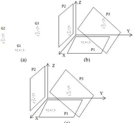
In the rigid transformation, one point cloud dataset is considered as the master and other datasets (i.e. the slave) will be registered to the master. In other words, all of the point clouds dataset will be registered to fixed pre-defined models (i.e. plane parameters). The unknown parameter vector of the least square adjustment consists of 3 rotation parameters and 3 translation parameters. These pre-defined models can be obtained from other datasets that have higher accuracy than the captured MLS point clouds (e.g. point clouds captured using TLS) or one of the captured point cloud in the project.Xiao et al. (2012) claimed that the transformation parameter can be calculated from three unparalleled planar surfaces. This requirement does not always assure the success of the transformation calculation. As shown in Figure 1: G1, G2 and G3 are three groups of points representing three different unparalleled surfaces P1, P2 and P3. As can be seen from the Figure 1 (b) and (c), there are more than one solution preserving the fitted on plane condition and the relative relationships between points. According to Skaloud and Lichti (2006), planes need to be vary in slope and orientation in order to assure the success of the least squares plane fitting adjustment. This requirement is too general. Theoretically, from the geometry point of view, the three rotation parameters can be computed from a pair of corresponding planes that is not parallel with any of the three axes (i.e. X, Y and Z axes) or from two corresponding pairs of planes parallel with two axes and intersect with each other. With respect to the calculation of the translation parameters, a pair of corresponding points is required. However, it is almost infeasible to find a pair of
“true” corresponding points in two different MLS point clouds, especially MLS sparse point clouds. Therefore, one of the requirements for the success of the least square adjustment is that there are at least a triplet of planes that intersect with each other and the intersection lines of them also intersect with each other at a points in the scene of the scan area. The more triplets present in the least square model, the stronger the least square model becomes. Moreover, the quality of the extracted planar surfaces that are used in the plane fitting model also plays a crucial part for the accuracy of the model’s outputs.
(a) (b)
(c)
Figure 1: (a) three groups of points; (b) and (c) two possible positions of points when fitting onto plane P1, P2 and P3
2.2 Plane detection algorithms 2.2.1 RANSAC
RANSAC proposed by (Fischler & Bolles, 1981) is possibly the most popular method used to detect and extract planes in laser scanning data due to its simplicity and robustness. It starts by randomly select three points, and then estimating the plane parameters based on these points. Next the orthogonal distances between points and the estimated plane are calculated. Points with distances smaller than a pre-defined threshold (od) will be labelled as “inlier” and form the consensus set. The process is iteratively repeated for a number of times. If the number of the largest consensus set is larger than a pre-defined threshold, this group will be considered as a planar feature. The outputs of RANSAC are heavily depended on the value of od. Furthermore, the spatial proximity between points is not taken into account leading to over and under-segmentation problems. According to Deschaud and Goulette (2010), RANSAC is not efficient in detecting small planar features. Further research has proposed a number of methods to improve the performance of RANSAC. In this research, the modified RANSAC method proposed by Previtali et al. (2014) was adapted to detect and extract planar features for the registration process. This method utilizes the normal vectors of points as well as the spatial proximity between points in detecting planar features.
2.2.2 Robust segmentation method based on robust diagnostic PCA (RDPCA)
with the lowest curvature value is chosen. Afterwards neighbouring points with similar normal vectors with that of the seed point and have orthogonal distances and Euclidian distances smaller than pre-defined thresholds are assigned to the current growing region. While the normal vectors difference threshold is defined by the user, the threshold for orthogonal and Euclidian distances are automatically estimated by the algorithm itself. Next each added point is used as the new seed point. The process is repeated until all of the points in the current region are used. Nurunnabi et al. (2015) proved that the performance of RDPCA is better than the region growing based on PCA (Rabbani et al., 2007) and RANSAC.
2.2.3 Plane detection based on line arrangement (Cabo) Cabo et al. (2015) prosed a method for detecting planar features in MLS point cloud based on scan profiles. First of all, different scan profiles are formed based on the scanlines information and the 3D version of the Douglas Peucker algorithm (Douglas & Peucker, 2011; Ebisch, 2002). Then a region growing based on these scan profiles is performed in order to detect and segment different planar surfaces. The longest scan profile is chosen as the seed point. There are three criteria for the region growing process of this method: neighbouring scan profiles (1) must be belong to the closest scanline of the seed scan profiles; (2) be parallel with each other; (3) the distance between them is smaller than a pre-defined threshold.
2.2.4 Region growing based on the planarity of the scan profiles (RGPL)
The plane detection and segmentation method proposed by Nguyen et al. (2016) utilizes the planarity of different groups of parallel scan profiles. It begins with splitting different scan lines into different scan profiles based on the direction vectors of points and distances between them. Then the planarity values of different groups of neighbouring parallel scan profiles are checked to form different planar features.
3. RESULTS AND DISCUSSIONS
Two datasets for the experiments were captured near the Curtin University Bentley campus in Australia using the Dynascan MDL S250 system (Renishaw, 2015). A part of the captured MLS point clouds (Figure 1) was used to investigate the accuracies of the matching processes using different segmentation approaches. Due to the specification of this MLS system, captured point clouds are sparse. The planar features with different sizes and orientations in this scanned area include vertical planes, horizontal planes and oblique planes (Figure 2).
In order to investigate the influence of different plane extraction approaches’ outputs, fifteen planar features were firstly manually extracted from the both captured datasets. The extracted planes from dataset 1 were used as the model, then, the transformation parameters were estimated by fitting the points on the corresponding planes extracted from dataset 2 to their correspondences in dataset 1. Then, the root mean square (RMS) errors of the planar features were also calculated. As the outputs from this process can be considered to be the most accurate, these calculated values were used as the benchmarks for comparisons.
(a)
(b)
(c)
(d)
(e)
(g)
Next, the experiments were separated into two parts. In the first part, the master were manually extracted from the dataset 1, the planar features in dataset 2 were extracted by using the discussed methods in section 2. In the second part, both of the
master and slave were automatically obtained by using the mentioned segmentation approaches. The experiments were implemented in C++.
3.1 Analysis of Scan area and plane fitting least square adjustment
Originally, most of the planar surfaces in this area are vertically orientated and are parallel with the vehicle’s trajectory directions (i.e. Y axis direction) and a group of planar surfaces is horizontal or near horizontal planes. They can be used to fix the translation along X direction and the translation along Z direction. However, they are insufficient to meet the requirements for the plane fitting least square adjustment discussed above (i.e. there are no triplet of plane that intersect at a point). Therefore, a target that has three planar surfaces was placed in the scan area (i.e. planes 1, 2 and 3 in Figure 3). As a result, detection of at least one of the two planar surfaces of the target (i.e. planes 1 and/or 3) is a must for the success of the registration of these two datasets. As plane 1 and 3 are quite small in term of the size and number of points. This will lead to more challenges for detection.
3.2 Benchmarks
Fifteen corresponding pairs of planar features were manually extracted from dataset 1 and 2 as shown in Figure 2. In this research, we assumed that those extracted planes are the best outputs from the captured datasets. Then, a least squares adjustment process that fit points on dataset 2 onto corresponding planar surfaces in dataset 1 was performed. In other words, dataset 1 is considered as the master and dataset 2 is considered as the slave. The estimated transformation parameters from this process are shown in Table 1. They were considered as the reference / benchmarking parameters.
(a)
(b)
Figure 3 Visualization of fifteen planar surfaces manually extracted from dataset 1
Rotations (°) Translations (m)
Ω Π Κ Tx Ty Tz
-0.190 -0.449 -0.004 -0.087 -0.256 -0.263 Table 1 Estimated transformation parameters of the
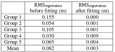
Besides comparing differences between the calculated transformation parameters of different approach with the benchmarks, the RMS values of the points of the data fitted to the corresponding surfaces residuals in the master for both before and after registration were calculated. In theory, the RMS of the residuals of points fitted on a plane will not be changed when the point clouds translate along any of the direction vectors of this plane. Therefore, in this experiment, benchmarking planar features were assigned into five groups based on their orientations. Group 5 consists of all the vertical planar features (i.e. 1, 4 and 6 to 14). Group 1, 2, 3 and 4 has only one planar feature namely 2, 3, 5 and 15 respectively. As can be seen from Figure 2, there are numbers of triplets of planes intersect to each other (e.g. plane 1, 15 and 4 or 3, 6 and 9, etc.) The requirement for plane fitting least square adjustment is met. As a result, the RMSregistration was reduced significantly from 82 mm to 3 mm after the least square plane fitting adjustment was performed. The RMS values of each group were calculated and evaluated (Table 2).
RMSregistration before fitting (m)
RMSregistration after fitting (m)
Group 1 0.155 0.000
Group 2 0.054 0.001
Group 3 0.105 0.001
Group 4 0.030 0.009
Group 5 0.065 0.004
Mean 0.082 0.003
Table 2 RMSs of the points fitted onto their models before and after least square adjustment process
3.3 Iterative closest point
Beside comparing the result of the least square plane fitting adjustment process using different input, this paper also compares the results of plane based fitting with point to plane approaches (Grant et al., 2012; Takai et al., 2013). According to Nguyen et al. (2016) the three nearest points point of the points are normally on the same scan line. Consequently, the point to plane approaches proposed by Grant et al. (2012) is not suitable for MLS point clouds. Hence, our paper adapts the point to plane approach proposed by Takai et al. (2013) for the experiment. The results show that the least square plane fitting adjustments provide the more accurate results (e.g. 0.003 m) for the registration process than the point to plane approaches (e.g. 0.022 m).
Rotations (°) Translations (m)
Ω Π Κ Tx Ty Tz
-0.122 -0.545 0.119 -0.086 -0.262 -0.020
Table 3 Estimated transformation parameters of point to plane
RMSregistration before fitting (m)
ICP RMSregistration after fitting (m)
Group 1 0.155 0.033
Group 2 0.054 0.003
Group 3 0.105 0.051
Group 4 0.030 0.016
Group 5 0.065 0.005
Mean 0.082 0.022
3.4 Registration between captured point cloud with the model (case 1)
In this part of our experiments, the benchmark was used as the
master for matching. Then, the four different segmentation approaches were applied in order to extract the corresponding surfaces in the dataset 2in which contains 15 planes Figure 4.
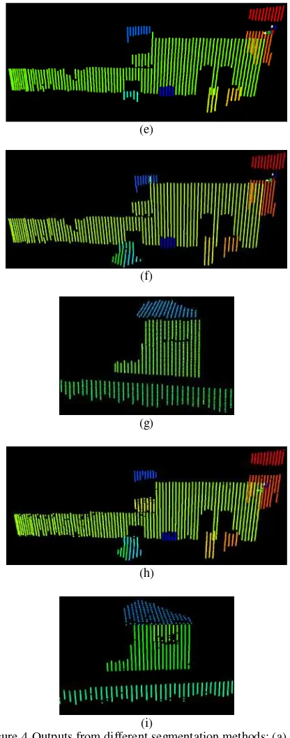
In the case of the plane extraction performed by using Cabo method, the numbers of detected corresponding features were twelve as: (1) surfaces 4 and 6 were assigned to the same features; (2) surfaces 13 and 14 were assigned to the same feature; and (3) the surfaces 2 and 3 were also detected as one feature. Meanwhile RANSAC, RDPCA and RGPL detected all of fifteen planar features. While the parameters for Cabo and RGPL were set similar to the suggested values in Cabo et al. (2014) and Nguyen et al. (2016) respectively, with RANSAC and RDPCA different parameters values were used to obtained the best outputs. The outputs of each segmentation method are showed in Figure 4. Based on these detected features, the corresponding plane pairs were specified based on distances and angles between features in two captured datasets. Finally, least square plane fitting adjustment processes were performed.
(a)
(b)
(c)
(d)
(e)
(f)
(g)
(h)
(i)
Figure 4 Outputs from different segmentation methods: (a) and (b) RANSAC; (c) and (d) RDPCA; (e) and (g) Cabo; (f) Cabo added; and (h) and (i) RGPL.
As can be seen from Figure 4, Cabo method failed in detecting plane 1 and 2 leading to the minimum requirement for the success of least square plane fitting adjustment process (see section 3) not being met. Consequently, there was a huge gap between the value of the estimated translation parameter along the Y direction and the benchmarking value. Figure 5 shows the point clouds of the target of after registration, significant horizontal differences are visible.
(a) (b)
Figure 5 (a) Top-back view of the target after registration; (b) front view of the target after registration
With the extracted planar features from RANSAC, RDPCA and RGPL, the requirement for the success of least square plane fitting adjustment was fulfilled. Consequently, it is not reasonable to compare Cabo with other methods in this case. Therefore, planar features 1 and 2 were added to the outputs of Cabo in order to perform a more reasonable comparison. Then, least square plane fitting adjustment processes with different inputs were performed.
The estimated transformation parameters of each method are shown in Table 3. Table 4 shows the differences between the estimated transformation parameters and the benchmark values.
Table 5 Estimated parameters from different segmentations methods
Table 6 Differences between the estimated values with the benchmark values
As shown in Table 4, the estimated transformation parameters using inputs from Cabo and RGPL were relatively close to the benchmark values. While there is a big gap between the estimated transformation parameters using RANSAC and RDPCA and the benchmarks. Different transformation parameters lead to differences in the accuracy of the registration processes. In order to evaluate the accuracy of the registration processes, the RMS values of the planes fitting residuals were calculated and shown in Table 5.
Theoretically, the objective of the least square adjustment method is to minimize the sum of the square of the residual of each equation in the model. Therefore, mean error values of
discrepancies of the transformation parameters and the RMS values of different methods,. Mean error value of each plane (ME) is calculated by using the following equation:
ME = xi * a + yi * b + zi * c – d
Where xi, yi and zi are the coordinates of point assigned to belong to plane
a, b, c and d are the plane parameters of the
benchmarks
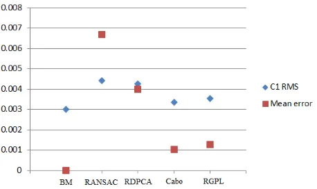
Planar features extracted by RDPCA and RANSAC have bigger mean errors than Cabo and RGPL (Table 6). Consequently, the registration outputs resulted from RDPCA and RANSAC have the worst RMS value among the four (e.g. 0.004 metre). Meanwhile, using inputs from RGPL and Cabo, the RMS values were improved by 25%. As a result, they are considered as the most accurate inputs for the least square plane fitting process in this case. Furthermore, the RMS values of these two methods approximate the benchmarking values. It is easy to see from Figure 8, the mean errors of the extracted planar surface used in the least square plane fitting adjustment are highly correlated with the RMS values of the final results (Figure 6) with the correlation coefficient value is 0.945. The lower the mean error is, the more accurate the final result is.
RANSAC
Table 7 RMSs after registration of four different approaches
RANSAC
Table 8 Mean error values of each group from three discussed segmentation methods
3.5 Registration between two captured point clouds (case 2)
In many projects, the references that can be treated as the
master for matching are not always available. Therefore, one of the captured point cloud is used as the master for registration. Hence, in this section, planar features in both of the master and
slave were automatically extracted by using the four mentioned segmentation methods. As can be seen from the least square plane fitting adjustment equation (equation 3), each inaccurate planar feature parameter contributes np number of inaccurate equation, where np is the number of points of the corresponding slave feature. Therefore, the accuracy of n and d values of each feature plays a very crucial part in the success of the least square adjustment model. Thus, the extraction of planar features for the master is more important than for the slave.
In order to evaluate the quality of the extracted features in the
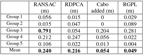
master, different descriptive measures of the bias angles (in degree) and distance to the origin (in metre) between benchmarks and the automatic extracted surfaces were calculated and are shown in Table 7 and Table 8. After segmentation, RGPL detects planar surfaces with the lowest differences compared with the benchmarks. On the other hand, RANSAC has the biggest differences in angles and distance to the origin, with mean values approximates 1.088 degree and 0.240 metre respectively. As the least square adjustment aims to minimize the sum of the square of the residual of each observation equation and the equations in the least square model are correlated to each other, in some case, a wrong equation can improve the residuals of other equations. Indeed, after registration, the mean RMS values of each process were similar like RMS values in case 1. For instance, the mean RMS value of RANSAC was approximate 0.004 metre in both cases. However, the RMS values of each group were changed. For instance, with RANSAC, the group 1 RMS value changed from 0.004 to 0.001. Table 9 the differences between angles of the surfaces extracted by the selected methods and the benchmarks
RANSAC Table 10 the differences between distances to the origin of the surfaces extracted by the selected methods and the benchmarks
In order to further investigate about the correlation between planes parameters and the RMS values of the registration process, another experiment was performed. In this
experiment, all of the model plane parameters were kept equal to the benchmark values except the parameters of plane in group 4 (plane 5 in Figure 3). The plane parameters for plane 5 were automatically extracted by using the discussed methods with the bias angle were 1624, 0.380, 0.633 and 0.282 degree by using RANSAC, RDPCA, Cabo and RGPL respectively. In this case, the result shows that there is also a very high correlation (e.g. 0.974) between the plane parameters and the final RMS values. Furthermore, if the difference is small (e.g. less than 1 degree in bias angle), the changes in final results is not significant.
Table 11 RMSs after registration of four different approaches with all automatically extracted features
RANSAC
Table 12 RMSs after registration of four different approaches in the case of group 4, feature was automatically extracted
4. CONCLUSION
Registration is one of the most important tasks in processing MLS point clouds. In this paper, we firstly discussed about the minimum requirement for the success of the least square plane fitting adjustment model for the MLS point clouds registration process. Then, three experiments were conducted on the outputs from four different state of the art planar segmentation methods: (1) RANSAC, (2) RDPCA, (3) Cabo and (4) RGPL. These four methods have different criteria to detect and extract planar features lead to differences in their outputs. The results of the registration process of MLS point clouds using least square plane fitting adjustment with planar features extracted by using these four methods are compared and presented. The results show that the accuracy of the registration process is highly correlated with the mean errors of the extracted planar features and the plane parameters. Among the discussed methods, RGPL and Cabo provide the highest accurate inputs for the registration process. However, Cabo cannot detect planar surfaces in the case they have similar orientation and are next to each other. RANSAC seems to be the worth among these 4 methods as its segmentation outputs have the biggest mean errors and differences in plane parameters. Furthermore, the least square plane fitting adjustment approaches seem to be better in registration of MLS sparse point clouds than the point to plane approach.
ACKNOWLEDGEMENTS
This research is supported by the Curtin International Postgraduate Research Scholarship (CIPRS)/Vietnamese Ministry of Education and Training – Vietnamese International Education Development Scholarship.
REFERENCES
Cabo, C., García Cortés, S., & Ordoñez, C. (2015). Mobile Laser Scanner data for automatic surface detection based on line arrangement. Automation in Construction, 58, 28-37. doi: http://dx.doi.org/10.1016/j.autcon.2015.07.005
Cabo, C., Ordoñez, C., García-Cortés, S., & Martínez, J. (2014). An algorithm for automatic detection of pole-like street furniture objects from Mobile Laser Scanner point clouds.
ISPRS Journal of Photogrammetry and Remote Sensing, 87(0),
47-56. doi: http://dx.doi.org/10.1016/j.isprsjprs.2013.10.008
Chan, T. O., & Lichti, D. D. (2012). CYLINDER-BASED SELF-CALIBRATION OF A PANORAMIC TERRESTRIAL LASER SCANNER. Int. Arch. Photogramm. Remote Sens.
Spatial Inf. Sci., XXXIX-B5, 169-174. doi:
10.5194/isprsarchives-XXXIX-B5-169-2012
Chan, T. O., Lichti, D. D., Belton, D., & Nguyen, H. L. (2016). Automatic Point Cloud Registration Using a Single Octagonal Lamp Pole. Photogrammetric Engineering & Remote Sensing, 82(4), 257-269. doi: http://dx.doi.org/10.14358/PERS.82.4.257
Chan, T. O., Lichti, D. D., & Glennie, C. L. (2013). Multi-feature based boresight self-calibration of a terrestrial mobile mapping system. ISPRS Journal of Photogrammetry and
Remote Sensing, 82(0), 112-124. doi:
http://dx.doi.org/10.1016/j.isprsjprs.2013.04.005
Deschaud, J.-E., & Goulette, F. (2010). A fast and accurate plane detection algorithm for large noisy point clouds using
filtered normals and voxel growing. Paper presented at the
Proceedings of the 5th International Symposium 3D Data Processing, Visualization and Transmission, Paris, France.
Douglas, D. H., & Peucker, T. K. (2011). Algorithms for the Reduction of the Number of Points Required to Represent a Digitized Line or its Caricature Classics in Cartography (pp. 15-28): John Wiley & Sons, Ltd.
Ebisch, K. (2002). A correction to the Douglas–Peucker line generalization algorithm. Computers & Geosciences, 28(8), 995-997. doi: http://dx.doi.org/10.1016/S0098-3004(02)00009-2
Fischler, M. A., & Bolles, R. C. (1981). Random sample consensus: a paradigm for model fitting with applications to image analysis and automated cartography. Commun. ACM, 24(6), 381-395. doi: 10.1145/358669.358692
Grant, D., Bethel, J., & Crawford, M. (2012). Point-to-plane registration of terrestrial laser scans. ISPRS Journal of
Photogrammetry and Remote Sensing, 72(0), 16-26. doi:
http://dx.doi.org/10.1016/j.isprsjprs.2012.05.007
Khoshelham, K., & Gorte, B. (2009). Registering point clouds
of polyhedral buildings to 2D maps. Paper presented at the
Proceedings of the 3rd ISPRS International Workshop.
Nguyen, H. L., Belton, D., & Helmholz, P. (2016). SCAN PROFILES BASED METHOD FOR SEGMENTATION AND EXTRACTION OF PLANAR OBJECTS IN MOBILE LASER SCANNING POINT CLOUDS. Int. Arch. Photogramm.
Remote Sens. Spatial Inf. Sci., XLI-B3, 351-358. doi:
10.5194/isprs-archives-XLI-B3-351-2016
Nurunnabi, A., West, G., & Belton, D. (2015). Outlier detection and robust normal-curvature estimation in mobile laser scanning 3D point cloud data. Pattern Recognition, 48(4), 1404-1419. doi: http://dx.doi.org/10.1016/j.patcog.2014.10.014
Previtali, M., Barazzetti, L., Brumana, R., & Scaioni, M. (2014). Scan registration using planar features. Int. Arch.
Photogramm. Remote Sens. Spatial Inf. Sci., XL-5, 501-508.
doi: 10.5194/isprsarchives-XL-5-501-2014
Rabbani, T., Dijkman, S., van den Heuvel, F., & Vosselman, G. (2007). An integrated approach for modelling and global registration of point clouds. ISPRS Journal of Photogrammetry
and Remote Sensing, 61(6), 355-370. doi:
http://dx.doi.org/10.1016/j.isprsjprs.2006.09.006
Renishaw. (2015). MDL Dynascan S250. Retrieved 21/07, 2015, from http://www.renishaw.com/en/dynascan-s250--27332
Skaloud, J., & Lichti, D. (2006). Rigorous approach to bore-sight self-calibration in airborne laser scanning. ISPRS Journal
of Photogrammetry and Remote Sensing, 61(1), 47-59. doi:
http://dx.doi.org/10.1016/j.isprsjprs.2006.07.003
Takai, S., Date, H., Kanai, S., Niina, Y., Oda, K., & Ikeda, T. (2013). Accurate registration of MMS point clouds of urban areas using trajectory. ISPRS Ann. Photogramm. Remote Sens. Spatial Inf. Sci., II-5/W2, 277-282. doi: 10.5194/isprsannals-II-5-W2-277-2013
Xiao, J., Adler, B., & Zhang, H. (2012, 13-15 Sept. 2012). 3D
point cloud registration based on planar surfaces. Paper
presented at the 2012 IEEE International Conference on Multisensor Fusion and Integration for Intelligent Systems (MFI).
Yang, B., Dong, Z., Liang, F., & Liu, Y. (2016). Automatic registration of large-scale urban scene point clouds based on semantic feature points. ISPRS Journal of Photogrammetry
and Remote Sensing, 113, 43-58. doi: