RECURSIVE LEAST SQUARES WITH REAL TIME STOCHASTIC MODELING:
APPLICATION TO GPS RELATIVE POSITIONING
F. Zangeneh-Nejad a, A. R. Amiri-Simkooei b, M. A. Sharifi a,*, J. Asgari b
a School of Surveying and Geospatial Engineering, Research Institute of Geoinformation Technology (RIGT), College of
Engineering, University of Tehran, Iran- (f.zangenehnejad, [email protected])
b Department of Geomatics Engineering, Faculty of Civil Engineering and Transformation, University of Isfahan, 81746-73441
Isfahan, Iran- (amiri, [email protected])
KEY WORDS: Recursive least squares, Stochastic modeling, Least-squares variance component estimation, GPS relative positioning
ABSTRACT:
Geodetic data processing is usually performed by the least squares (LS) adjustment method. There are two different forms for the LS adjustment, namely the batch form and recursive form. The former is not an appropriate method for real time applications in which new observations are added to the system over time. For such cases, the recursive solution is more suitable than the batch form. The LS method is also implemented in GPS data processing via two different forms. The mathematical model including both functional and stochastic models should be properly defined for both forms of the LS method. Proper choice of the stochastic model plays an important role to achieve high-precision GPS positioning. The noise characteristics of the GPS observables have been already investigated using the least squares variance component estimation (LS-VCE) in a batch form by the authors. In this contribution, we introduce a recursive procedure that provides a proper stochastic modeling for the GPS observables using the LS-VCE. It is referred to as the recursive LS-VCE (RLS-VCE) method, which is applied to the geometry-based observation model (GBOM). In this method, the (co)variances parameters can be estimated recursively when the new group of observations is added. Therefore, it can easily be implemented in real time GPS data processing. The efficacy of the method is evaluated using a real GPS data set collected by the Trimble R7 receiver over a zero baseline. The results show that the proposed method has an appropriate performance so that the estimated (co)variance parameters of the GPS observables are consistent with the batch estimates. However, using the RLS-VCE method, one can estimate the (co)variance parameters of the GPS observables when a new observation group is added. This method can thus be introduced as a reliable method for application to the real time GPS data processing.
* Corresponding author
1. INTRODUCTION
The least squares (LS) parameter estimation has been extensively employed in geodetic data processing. There are two different forms for the LS namely batch form and recursive LS (RLS) form. In the batch form, the whole measurements are simultaneously processed through the adjustment procedure while the RLS processes the observations sequentially in time. The RLS method is therefore suitable for real time applications in which observations are collected sequentially over time. To obtain the best linear unbiased estimation (BLUE) using the least squares method, either in batch form or in recursive form, the realistic choice of the stochastic model of the observables is an essential issue. This describes the statistical properties of observables by means of a covariance matrix. The covariance matrix of observables is relatively known and expressed as an unknown linear combination of known cofactor matrices for most geodetic applications. The estimation of the unknown (co)variance parameters is referred to as variance component estimation (VCE). There are many different methods for VCE such as best invariant quadratic unbiased estimator (BIQUE) (Koch 1978, 1999), minimum norm quadratic unbiased estimator (MINQUE) (Rao 1971 and Junhuan et al 2011),
restricted maximum likelihood (REML) estimator (Koch, 1986) and the least squares variance component estimation (LS-VCE) (Teunissen 1988; Teunissen and Amiri-Simkooei 2006, 2008 and Amiri-Simkooei 2007).
GPS data processing is usually performed using the LS method in a recursive manner via a sequential filter, i.e., a least squares sequential filter or discrete Kalman filter. A realistic stochastic model for the GPS observables is therefore necessary for high-precision GPS positioning. The noise characteristics of GPS observables has been investigated by Amiri-Simkooei and Tiberius (2007), Amiri-Simkooei et al. (2006, 2007, 2009, 2013), Bischoff et al. (2006), Tiberius and Kenselaar (2000, 2003), Teunissen et al. (1998), Hartinger and Brunner (1999), Wang et al. (1998, 2002), and Satirapod et al. (2002). Amiri-Simkooei et al. (2009, 2013) have been applied the LS-VCE algorithm to GPS observables using the geometry-free observation model (GFOM) and the geometry-based observation model (GBOM), respectively. They applied the LS-VCE to the GPS observables in a batch form. This causes the high computational time needed for the batch solution. To overcome such a problem, the entire time span of the GPS observations was divided into a few groups, each consisting of a few consecutive epochs. The unknown (co)variance parameters
(k;k 1 : )p can then be separately estimated for each group using the LS-VCE method. For a Kronecker and block structure of the functional and stochastic models, one can show that the final estimates are just the arithmetic mean of the individual estimates over the groups.
In the case of GPS data processing, the stochastic model can represent unmodeled systematic errors, multipath and noise. Therefore to adapt the stochastic model with the environment, the stochastic model must be properly chosen in real time so that the unknown parameters and the stochastic model are both updated as new data arrive over time. In this contribution, we look for a recursive procedure providing a proper stochastic modeling for GPS observables using the LS-VCE method. This paper is organized as follows. The RLS method is first introduced and described in details in the next section. We then explain how the recursive LS-VCE is implemented in GPS relative positioning. In order to assess the noise characteristics of GPS observables, the implementation results of the proposed method are then provided and compared with those obtained by the batch solution. Finally we draw some conclusions in the last section.
2. RECURSIVE LEAST SQUARES (RLS) The RLS is an appropriate method for sequential rather than batch processing. Consider the following partitioned linear model of observation equations:
1
corresponding design matrices, respectively, and
1 respectively. The correlation between
y
1 andy
2 is assumed to be absent (i.e.1 2
0 y y
Q ).
The model of observation equations in Eq. (1) is also equivalent to the following model (Teunissen 2000)
1 The recursion of the LS solution of Eq. (2) is then of the form (Teunissen 2000, 2001, 2005) subsection, the GBOM model is briefly explained, which here is considered to be the functional model for assessing the noise characteristics of GPS observables in a recursive manner.
2.1 GPS Geometry-Based Observation Model (GBOM)
The GBOM model is a commonly used model for high-precision GPS positioning from code and phase observations using a relative GPS receiver setup. In the model, the observations are the DD pseudorange and phase observation on the L1 or L2 frequency. The unknown vector consists of the unknown baseline components between the reference and rover receivers and the DD integer ambiguities on the L1 or L2 (Teunissen, 1997, Odijk 2008 and Amiri-Simkooei et al. 2013). Ignoring the DD atmospheric (ionospheric and tropospheric)
delays, the observation equations of the GBOM at epoch
t
k is of the form pseudorange and phase observations between two receivers andtwo satellites on the L1 or L2 frequency, respectively,
A
k is the design matrix, the vector g consists of the unknown baseline components between the reference and rover receivers and a is the vector of DD integer ambiguities on the L1 or L2.At first, the unknowns of Eq. (6) are obtained using some initial epochs. The unknown vector can then be updated using Eqs. (3-5) recursively when new observations related to the consecutive epochs are added.
2.2 A realistic stochastic model of GPS observables
The complete structure of stochastic model of the GPS observables considering different variance components for observables (C1, P1, L1 and L2), correlations among observations, satellites elevation dependence of GPS observables precision and temporal correlations of observables is of the form (Amiri-Simkooei et al. 2009; 2013)
D
representing time correlation of the observables (K is the epochs of observations).
describing the satellite elevation dependence of GPS observables precession (k is the number of satellites, and the satellite number [1] is assumed to be the reference satellite).
Table 1 Matrices
C,
T and
E given in Eq. (7)In this contribution, the time correlation of observations is
ignored, i.e.,
TI
K whereI
K is an identity matrix of sizeK. However, to consider the satellites elevation effect on the GPS observables precision, an elevation-angle based sine function model is employed as follows
2 procedure providing a proper stochastic modeling for GPS observables using the LS-VCE method.
3. LEAST-SQUARES VARIANCE COMPONENT vector l are given as (Amiri-Simkooei 2007)
1 1 variances of the estimates
ˆ
is also expressed by the diagonal entries of the covariance matrix of the estimated (co)variancecomponents, which is obtained as Q N1. For more
information about LS-VCE we refer to Teunissen and Amiri-Simkooei (2008) and Amiri-Amiri-Simkooei (2007).
3.1 Application of LS-VCE to GPS observables stochastic modelling
The covariance matrices of the observables should be properly defined for high-precision GPS positioning applications. We aim to assess the noise characteristics of the GPS observables using the GBOM in a recursive manner.
To obtain the realistic stochastic model of the GPS observables,
one should properly determine the three matrices
C,
T andE
given in Eq. (7). In this contribution, the time correlation ofobservations is ignored, i.e.,
TI
K and the satellites elevation effect on the GPS observables precision is modeled using an elevation-angle based sine function given in Eq. (8),i.e., the matrix
E is also known. However, the components ofthe matrix
Care estimated using the LS-VCE method. These (co)variance parameters (here the components of thematrix
C) can then be separately estimated for each group. The final estimates of the unknown (co)varianceparameters are just the arithmetic mean of the individual observations is added. Further descriptions are given hereinafter.
3.2 Application of recursive LS-VCE to GBOM model In the first step, assume
Q
, respectively. The components of the matrix
C (4 variances and 6 covariances) can also be obtained using the LS-VCE method.Assuming the new group of observations is also added to the problem. Now again consider the following partitioned model of observation equations which is equivalent to the model of observation equations of Eq. (1)
1
The unknown components of the matrix
C (4 variances and 6 covariances) can also be obtained using the LS-VCE as1
ˆ N l
where N and l are given by Eqs. (10 and 11). Note that in the batch method, these parameters are obtained for each group of observation, separately, i.e., we used only main difference of the method with the batch method. Similarly, the final estimates of the unknown (co)variance parameters are the arithmetic mean of the individual estimates over the groups.
4. RESULTS AND DISCUSSIONS
To apply the RLS-VCE method, we used one zero baseline GPS data set. The receiver used in this experiment is Trimble R7 corresponded to January 1th, 2004, from 12:25:00 to 13:15:00 UTC. The total number of epochs is then 3000. The data set is collected at a meadow area close to Delft, the Netherlands with 1-sec intervals providing the code and phase observations on both the L1 and L2 frequencies (namely, C1–P2–L1–L2). The noise characteristics of GPS observations are now investigated for both batch and recursive solution procedures. This section consists of two subsections. In the first part, the
variances of the GPS observables for C1, P2, L1 and L2 observables are provided. The covariances/correlations among the GPS observables are given in the second subsection.
4.1 Variances of GPS observables
whereas the off-diagonal elements are the covariances between the observables.
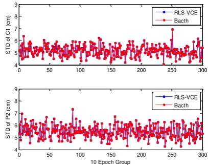
At first, the entire time span of the GPS observations for the data set we used is divided into 300 groups, each consisting of a 10 consecutive epochs. The (co)variance parameters can then be estimated using the LS-VCE method in a batch manner or in a recursive manner. Applying the LS-VCE in a batch form, one can obtain the (co)variance parameters for each group of observations (here 300 groups) separately. In the recursive form, the (co)variances parameters can be estimated recursively when the new group of observations is added. Use is made of the model given in Eq. (13). Figures 1 and 2 show the groupwise estimate of the standard deviations of C1 and P2 and L1 and L2 for the Trimble R7 receiver, respectively, for both batch and recursive solutions. The results confirm the consistency between the batch estimates and the recursive ones. However, applying the LS-VCE method in a recursive manner provides a real time stochastic modeling for GPS observables as new data arrive over time. This is a great advantage of the RLS-VCE compared to the batch one.
0 50 100 150 200 250 300
Fig. 1 Estimated standard deviations of GPS code observations (C1 and P2) for Trimble R7 receiver in cm for both batch and
recursive methods
For a better view, the estimated standard deviations of four GPS observation types for both solutions are presented in Table 2 (in mm). As mentioned, the final estimates of the unknown (co)variance parameters are just the arithmetic mean of the individual estimates over the 300 groups for both batch and recursive methods.
0 50 100 150 200 250 300
Fig. 2 Estimated standard deviations of GPS phase observations (L1 and L2) for Trimble R7 receiver in mm for both batch and
recursive methods
Table 2 Estimated standard deviations of four GPS observation types for both solution forms in mm
Method C1 P2 L1 L2
Batch 51.7 55.1 0.8 0.9
RLS-VCE 51.8 55.1 0.8 0.9
4.2 Correlations among GPS observables
According to the description provided in the previous section, the covariances/correlations among the GPS observables are estimated using the LS-VCE method in both batch and recursive forms. We estimated the six correlations among C1 and P2, C1 and L1, C1 and L2, P2 and L1, P2 and L2 and L1 and L2, among them , for example, figure 3 provides the estimated correlations among the phase observations L1 and L2ferquencies for Trimble R7 receiver using both batch and recursive methods. The results indicated a significant correlation between the phase observations L1 and L2 of about 0.9 for Trimble R7 receiver. Similarly again, the consistency
Fig. 3 Estimated correlations among phase observations on L1 and L2 frequencies for Trimble R7 receiver for both batch and
recursive methods
5. CONCLUDING REMARKS
The least squares (LS) adjustment procedure can be extensively used in geodetic data processing in two different but equivalent forms: 1) batch form and 2) recursive least squares (RLS) form. For real time applications in which observations are collected sequentially over time, the RLS method is preferred compared to the batch one. Concerning the LS adjustment method either in batch form or in recursive form, both functional and stochastic models should be properly defined. The realistic choice of the stochastic model of the observables is required to obtain the best linear unbiased estimation (BLUE). This is important for GPS data processing as well. The model we used here is the geometry-based observation model (GBOM). The model consisting of two parts: the functional and the stochastic models. The former is completely established. Therefore, the choice of the functional model for the GPS observables is not the subject of discussion in this contribution. However, choosing a realistic stochastic model for the GPS observables is necessary for high-precision GPS positioning which was the subject of the research. At first, the covariance matrix of observables has been expressed as an unknown linear combination of known cofactor matrices. The unknown (co)variance parameters can then be estimated using the different variance component estimation (VCE) methods. Here, we investigated the noise characteristics of the GPS observables using the least squares variance component estimation (LS-VCE) method. The LS-VCE algorithm can be implemented to GPS observables in a batch manner or in a recursive manner. The former has already been investigated by Amiri-Simkooei et al. (2009, 2013). We proposed a recursive procedure providing a proper stochastic modeling for GPS observables using the LS-VCE method.
To consider the performance of the proposed method and to access the proper GPS observable covariance matrix, real data, collected by one GPS receiver Trimble R7 was used. We employed the LS-VCE algorithm on the GPS observations for the two different cases batch and recursive forms. Applying the LS-VCE in a batch form, one can obtain the (co)variance parameters of the GPS observables for each group of observations separately. In the recursive form, the (co)variances parameters can be estimated recursively when the new group of observations is added. This is a great advantage of the RLS-VCE rather than the batch one. The results confirmed that the proposed method has an appropriate performance so that the estimated (co)variance parameters of the GPS observables are completely consistent with the batch estimates. This method can thus be introduced as an efficient method to the GPS processing stage.
REFERENCES
Amiri-Simkooei, A.R., 2007. Least-squares variance component estimation: Theory and GPS applications. Ph.D. thesis, Delft Univ. of Technology, Delft, The Netherlands.
Amiri-Simkooei, A.R., Tiberius, C.C.J.M., and Teunissen, P.J.G., (2006). Noise characteristics in high precision GPS positioning. P. Xu, J. Liu, A. Dermanis, eds., Proc., 6th Hotine-Marussi Symp. of Theoretical and Computational Geodesy, Springer, Berlin, pp. 280–286.
Amiri-Simkooei, A.R., and Tiberius, C.C.J.M., 2007. Assessing receiver noise using GPS short baseline time series. GPS Solutions, 11(1), pp. 21–35.
Amiri-Simkooei, A.R, Teunissen, P.J.G., Tiberius, C.C.J.M., 2009. Application of least-squares varinace component estimation to GPS observables. J Surv Eng., 135(4): pp. 149-160.
Amiri-Simkooei, A.R., Zangeneh-Nejad, F., and Asgari, J., 2013. Least-squares variance component estimation applied to GPS geometry-based observation model. J Surv Eng., 139(4): pp. 176-187.
Bischoff, W., Heck, B., Howind, J., and Teusch, A., 2006. A procedure for estimating the variance function of linear models and for checking the appropriateness of estimated variances: A case study of GPS carrier-phase observations. J. Geodesy, Berlin, 79(12), pp. 694–704.
Hartinger, H., and Brunner, F. K., (1999). Variances of GPS phase observations: The SIGMA- model. GPSSolutions, 2(4), pp. 35–43.
Junhuan, P., Yun, S., Shuhui, L., and Honglei, Y., 2011. MINQUE of variance-covariance components in linear Gauss-Markov models. J. Surv. Eng., 137(4), pp. 129–139.
Koch, K.R., 1978. Schätzung von varianzkomponenten. Allgemeine Vermessungs-Nachrichten, 85: pp. 264–269.
Koch, K.R., 1986. Maximum likelihood estimate of variance components. Boll. Geod. Sci. Affini, 60: pp. 329–338. (Ideas by A.J. Pope).
Koch, K.R., 1999. Parameter estimation and hypothesis testing in linear models. Springer Verlag, Berlin.
Odijk, D., 2008. GNSS Solutions: What does geometry-based and geometry-free mean in the context of GNSS? Inside GNSS,
3(2), pp. 22–24.
Rao, C.R., 1971. Estimation of variance and covariance components - MINQUE theory. Journal of multivariate analysis, 1(3): pp. 257–275.
Satirapod, C., Wang, J., and Rizos, C., 2002. A simplified MINQUE procedure for the estimation of variance-covariance components of GPS observables. Survey Rev., 36(286), pp. 582–590.
Teunissen, P.J.G., 1997. The geometry-free GPS ambiguity search space with a weighted ionosphere. J. Geodesy, Berlin, 71(6), pp. 370-383.
Teunissen, P.J.G., 1988. Towards a least-squares framework for adjusting and testing of both functional and stochastic model. Internal research memo, Geodetic Computing Centre, Delft. A reprint of original 1988 report is also available in 2004, No. 26.
Teunissen, P.J.G., Jonkman, N.F., and Tiberius, C.C.J.M., 1998. Weighting GPS dual frequency observations: Bearing the cross of cross-correlation. GPS Solutions, 2(2), pp. 28–37.
Teunissen, P.J.G., 2000. Adjustment theory: an introduction. VSSD: Delft University Press. Series on Mathematical Geodesy and Positioning.
Teunissen, P.J.G., 2001. Dynamic data processing: Recursive least-squares. VSSD: Delft University Press. Series on Mathematical Geodesy and Positioning.
Teunissen, P.J.G., Simons, D.G., and Tiberius, C.C.J.M., 2005.
Probability and observation theory. Delft: Delft University of Technology.
Teunissen, P.J.G., and Amiri-Simkooei, A.R., 2006. Variance component estimation by the method of least-squares. Proc., 6th Hotine-Marussi Symp. of Theoretical and Computational Geodesy, IAG Symposia, Vol. 132, P. Xu, J. Liu, and A. Dermanis, eds., Springer, Berlin, 273–279
Teunissen, P.J.G., and Amiri-Simkooei, A.R., 2008. Least-squares variance component estimation. J. Geodesy, Berlin, 82(2), pp. 65–82
Tiberius, C.C.J.M., and Kenselaar, F., 2000. Estimation of the stochastic model for GPS code and phase observables. Survey Rev., 35(277), pp. 441–454.
Tiberius, C.C.J.M., and Kenselaar, F., 2003. Variance component estimation and precise GPS positioning: Case study.
J. Surv. Eng., 129(1), pp. 11–18.
Wang, J., Stewart, M.P., and Tsakiri, M., 1998. Stochastic modeling for static GPS baseline data processing. J. Surv. Eng.,
124(4), pp. 171–181.
Wang, J., Satirapod, C., and Rizos, C., 2002. Stochastic assessment of GPS carrier phase measurements for precise static relative positioning. J. Geodesy, Berlin, 76(2), pp. 95–104.