Vehicle Routing Problem with Backhaul,
Multiple Trips and Time Window
Johan Oscar Ong1, Suprayogi2
Abstract: Transportation planning is one of the important components to increase efficiency and effectiveness in the supply chain system. Good planning will give a saving in total cost of the supply chain. This paper develops the new VRP variants’, VRP with backhauls, multiple trips, and time window (VRPBMTTW) along with its problem solving techniques using Ant Colony Optimization (ACO) and Sequential Insertion as initial solution algorithm. ACO is modified by adding the decoding process in order to determine the number of vehicles, total duration time, and range of duration time regardless of checking capacity constraint and time window. This algorithm is tested by using set of random data and verified as well as analyzed its parameter changing. The computational results for hypothetical data with 50% backhaul and mix time windows are reported.
Keywords: Vehicle routing problem, vehicle routing problem with backhauls, multiple trips, time window, sequential insertion, ant colony optimization, ant system.
Introduction
The Transportation cost is one of component cost in logistic system which has dominated total cost wholly. This transportation cost must be efficient in order to give contribution for decreasing total cost and increasing the firm’s competitive advantage. Finding efficient vehicle routes and its schedule are a representative logistics problem. Vehicle routing pro-blem (VRP) goals to find a set of tour for several vehicles from a depot to a lot of customers and return to the depot without exceeding the capacity
con-straints of each vehicle at minimum cost (Bin et al.
[1]). Brandao [2] defines more specific that is distri-buting products to number of customers in certain region with deterministic demand.
Various types of VRP model have been developed to accommodate various real situations. Suprayogi [14] explained it such as VRP with time windows (VRP-TW), VRP with multiple trips (VRPMT), and VRP with simultaneous pick-up delivery (VRPPD). There is a specific variant that discusses the separating service between linehauls customer and backhaul customer, VRP with backhauls (VRPB). Generally, VRPB can be classified as two types of problem; those are VRPB with customer priority and VRPB
without customer priority (Tavakkoli-Moghaddam et
al. [15]).
1 Faculty of Industrial Teknology, Industrial Engineering
Department, Institut Teknologi Harapan Bangsa. Jl. Dipatiukur 80-84, Bandung 40132. Email: [email protected].
2 Faculty of Industrial Technology, Industrial Engineering
Department, Bandung Institute of Technology, Jl. Ganesha 10, Bandung 40132. Email: [email protected]
Received 19 January 2011; revised1 28 February 2011; revised2 15 March 2011; Accepted for publication 30 March 2011.
Crispim et al. [6] explained that VRPB has same
constraint with VRP but there is an addition constraint, linehauls customers are served before backhaul customers. VRPB model must be adjusted with real condition that considers multiple trips and time window, VRPBMTTW. The example problem for this variant is finding the vehicle routes for chemical distributors. Distributors have to deliver chemical substances to a lot of agents and retailers which spread at certain area. Distributors also have to pick up the chemical substances from suppliers. The separation between linehauls and backhaul is caused by hazardous chemical substances that cannot be put together at the same vehicle.
A number of vehicles are assigned to deliver chemical substances and after that, the vehicles are assigned to pick up chemical substances. This service can be done in the time window and certain planning horizon, as well as vehicles are allowed to go back and forth to distributor for loading and unloading chemical substances.
Various techniques have been developed to solve
VRP. Bin et al. [1] said that VRP is a hard
combina-torial problem. Consequently, VRP is generally solved by using heuristic and meta-heuristic approach, such as 2 opt, 3 opt, simulated annealing, genetic algorithm, tabu search, ant colony optimiza-tion, etc.
Now, metaheuristic approach is mainly used because of its ability to solve the problem more intensively. Ant colony optimization (ACO) is one of the metaheuristic approaches that can be used to solve hard combinatorial problems. Dorigo and Blum [10] concluded that ACO gives a good solution in short
vehicle routing problems, sequential ordering problems, resource constraint problems, and open shop scheduling problems. Mong Sim and Hong Sun [12] also said that ACO results good solution for routing and balancing problem. In his research, Bell and McMullen [3] explained that ACO results good solution for VRP. ACO gives good solution and efficient enough for very complex problem (Doerner
et al.[7]).
There are two general ways to generate VRP initial solution, those are using savings criterion and inserting customer sequentially to the route with cost criteria (Laporte et al. [11]). Sequential inser-tion is often used to solve vehicle routing problem because it is easy to be modified to accommodate complex constraints.
Methods
VRP with Backhaul and Time Window (VRPB-TW)
VRPB-TW model is a model developed from the basic model VRPB by adding constraint of time window on each customer. Cho and Wang [5] developed a model VRPB-TW that minimize the amount of vehicles and routing time by starting from the depot and ends at the depot. The VRPB-TW consists of finding a set of vehicle routes with a lot of constrains, such that: (1) each vehicle services one
route; (2) each customer node i is visited exactly
once; (3) the quantity of goods on-board never exceeds the vehicle capacity; (4) the linehauls customers precede the backhauls on each vehicle route; (5) the start time on each vehicle route is greater than or equal to the time window’s lower bound at depot; (6) the return time on each vehicle route is less than or equal to the time window’s upper bound at depot; (7) the time of beginning of service at each node i is less than or equal to the time
window’s upper bound li; and (8) the time of
beginning of service at each vertex i is greater than
or equal to the time window’s lower bound ei. Cho
and Wang [5] solve this model with metaheurisic technique threshold accepting (TA). Unlike Zhong and Cole [16] complete with local search techni-ques for similar problems.
VRP with Multiple Trips, Time Window, and Pickup Delivery (VRP-MTTWPD)
VRPMTTWPD is a combination of variants vehicle routing problem with multiple trips (VRPMT), vehicle routing problem with time window
(VRP-TW), and vehicle routing problem with pickup
delivery (VRPPD). The characteristics of VRPMTT-WPD model is that each customer has a
time-win-dow, each vehicle can have more than one route
during the planning horizon, and the customer
receives the supply of goods from the depot and send the goods to the depot. These models will get a set of tours that meet the delivery demand and also pickup demand (Suprayogi and Priyandari [13]).
There are three objectives to be achieved on the model VRPMTTWPD, i.e, minimize the number of tours, total tour duration time, and a range of duration time of the langest and shortest tour. The number of tour represents capital cost that is mini-mized, labor cost and other operating costs. Total duration time represents vehicle operiational cost, e.g., fuel consumption. Total tour duration time represents the minimization of operational costs of vehicles, fuel samples. Generally, these objectives are usually found in the vehicle routing problem model. The third objective represents a balance total duration time of each tour. Suprayogi and Priyandari [13] solved this model by using genetic algorithm and tabu search.
Each of these goals is weighted W1, W2 and W3.
While, W1 > W2 > W3 reflects that the first goal has
greather priority than the second one, and the second goal has a greater priority than the third one. We set W1: 100000, W2 : 100, W3 : 0.00005 with the
objective function as:
· · · (1)
Result and Discussion
System Description
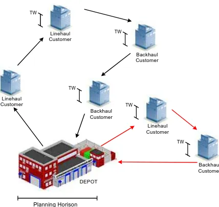
In this paper, the system is defined as system that connected with finding set of tour for several vehicles in distributing products. This system consists of a depot, linehauls customers, and backhaul customers. Every activities starts from depot and ends to the depot. For every customer and depot, there is loading/unloading time. The unit measurement for loading/unloading time is same as unit measure-ment for customer’s demand. Figure 1 shows the representation of system structure. In a planning horizon, one vehicle can serve more than one customer starting linehauls customer and after that backhaul customer. One vehicle can serve more than one route, only same product each delivery, and only at customer’s time window.
Figure 1. System architecture
Backhauls can be defined as vehicle serves customer in a route apart from pick up activity and delivery activity. Delivery customers (linehauls customer) are served first before pick up customers (backhauls customer).Vehicle serves a set of routes in every tour, is called multiple trips, and returns to depot before serving others route. This condition can only be fulfilled if service time is in planning horizon. Vehicle goes to customer in a certain time window that has been stated before and also deterministic demand. This constraint makes vehicle waiting if it has arrived before the time windows. Time window is an interval time that customers provide to accept the service. In this research, there are loading and unloading times which respectively represent the time to move goods from warehouse to vehicle and just the opposite. The loading and unloading time will not exceed initial service time and the end of service time.
This model considers the customer’s priority which linehauls customer serves before backhauls custo-mer. The objective functions are to minimize the number of vehicles, minimize total tour completion time, and minimize range of duration time. We find the solution lexicographically or alphabetically. It means that the objective function are given priority consecutively, which the first objective has higher priority than the second objective and the third objective.
Decision variables are number of tours, customer’s sequence served in every route and tour, arrive time, earliest service time, latest service time, and departure time at every customer. The parameters are number of linehauls customer, a number of backhauls customers, linehauls customer’s demand, backhauls customer’s demand, distance, vehicle’s speed, time window, and planning horizon.
There are a lot of constraints in vehicles routing problem with backhaul, multiple trips, and time window (VRPB-MTTW):
(i) Every route starts and ends at depot
(ii) Planning horizon indicates the starting and the
ending of vehicle activity
(iii) Delivery demand and pickup demand are
deterministic and known.
(iv) Vehicle serves backhauls customer after
linehauls customer
(v) Every customer can only be served once by one
vehicle.
(vi) The vehicle’s load must not exceed vehicle’s
capacity
(vii) Service time can only be started at earliest
time and before or equal with latest time
Range of Duration Time (RDT) is a difference between the longest tour duration time and the shortest tour duration time
, : number of linehauls customers’
posi-tions in route from tour
, : number of backhaul customers’ positions
in route from tour
, , : earliest departure time at node position
in route from tour
, , : latest departure time at node position
in route from tour
, , : starting time for service at node position
in route from tour
, , : earliest starting time for service at node
, , : latest starting time for service at node position in route from tour
, , : waiting time at node position in route
from tour
, : Total delivery load in route r from tour
, : Total pick-up load in route from tour
, , : Total load at position in route from
tour
, , : Loading-unloading time at position in
route from tour
Parameter:
, : travel time from node to : earliest time window at node
: latest time window at node : delivery demand at node with : pick up demand at node with
: vehicle capacity : service time
: number of linehauls customer : number of backhauls customer
Performance criteria:
NV : number of vehicles
TDT : total duration time
RDT : difference between the longest tour duration time and the shortest tour duration time
Every , , location for certain , and refers to
node , thus
, , (2)
To assure that every node can only visited exactly
once, every appears once at certain , and ,
except for . Therefore, this can be stated as:
, , (3)
From this equation onward, we use these following indexes; instead they are stated differently.
, , … , ; , , … ,
, , … , ,
, , (4)
Total delivery and pickup load for any route can be stated respectively as:
, ∑NL , , , k (5)
, ∑NL , , , k (6)
Total load in vehicle for any location can be stated recursively as:
, , , , , , (7)
, , , , , , (8)
and
, , , (9)
, ,
, , , , … , , (10)
The vehicle’s capacity constraint can be expressed in the following inequalities:
, (11)
, (12)
To make sure that linehauls customer must be served before backhaul customer, can be expressed in the following equality:
∑ ∑ , , , (13)
Earliest arrival time, starting time for service and earliest departure time at location can be determined by forward counting as follow:
, , , , , , , , , (14)
, , max , , , , , (15)
δ , , σ , , s , , (16)
with
, , (17)
α , , δ , , , (18)
The visibility of time window can be stated as:
, , , , (19)
for equation (15), (16) and (19) , , … , ,
Loading/unloading time at any node for linehauls customer is the total delivery demand at that node and as well as for backhauls customer, as follow:
, , , , (20)
s , , , , (21)
Especially for node 0 (depot), loading/unloading time from depot and ends to depot can be stated as:
, , , (22)
s , , , , (23)
Latest arrival time time and latest departure time at any location is determined by backward counting as follow:
, , , , , , (24)
, , , , , (25)
, , … ,
, , , , , (26)
so that, the expression can be stated as: , , , , , (27)
, , , , (28)
, , , , (29)
, , , , (30)
For equation (26) and (27) , , … , ; meanwhile for equation (28)-(30) , , … , , Waiting time for any location is represented in the following expression: , , , , , , , , , , , , if , , , , , … , , 31 Tour duration time is defined as difference between the arrival time (starting time for service) at the depot for the first time and the departure time (ending time for service) at the depot for the last time. This can be expressed as: , , , , , , … , , The total tour duration time is a summation of all tour duration times stated as: ∑ (33)
Range of Duration Time (RDT) is defined as a difference between the maximum of tour duration time and the maximum of tour duration time, is formulated as follow: , , (34)
RDT will be set zero if there is only one vehicle to serve all customers. Every vehicle can only serve exactly one tour. Thus, number of vehicles used is equal to number of tours. This can be stated as: (35)
This model has three objectives preference struc-tures considered. For all strucstruc-tures, minimizing number of vehicles (NV) is always place as first objective. The second objective is minimizing the total duration time (TDT) and the last is minimizing range of duration time (RDT). Therefore, It can be formulated as: , , (36)
Solution Approach
Various techniques both optimal and heuristics have been developed to solve the vehicle routing problem. Bullnheimer et al. [4] stated that the vehicle routing problem is a hard combinatorial problem with a computational combinatorial increased along the increasing size of the problem. Vehicle routing pro-blem is generally solved with heuristic and meta-heuristic approach e.g. 2 opt, 3 opt, simulated annea-ling, genetic algorithm, tabu search, ant colony optimization, etc.
Sequential insertion is the most often used method in solving vehicle routing problems. This is caused by the speed in delivering solution, easy to use and easily modified to handle a difficult constraint. Sequential insertion algorithm is used to generate the initial feasible solution. First, algorithm will generate a tour and the first route. Algorithm chooses linehauls customer by using predetermined rule. These rules are earliest deadline, earliest ready time, shortest time window, and longest travel time.
Steps of the sequential insertion algorithm are described as follows.
Step 0:
Input all the parameters and initialize the set of unassigned linehauls customer and the set of
unassigned backhauls customer . Go to step 1.
Step 1:
Create a tour and a route of this tour by setting
and , starts from depot.
Step 2:
As long as there are unassigned linehauls customers , do this step. If all linehauls custo-mers have been
served, go to step 9. For and , choose
unassigned linehauls customers as seed customer
using predeter-mined rule. Then go to step 4.
If , then go to step 3.
Step 3:
Step 4:
Check the feasibility of time window for linehauls customer . If it is feasible, then insert customer and calculate the load after exit from customer . Then go to step 5. If time window is not feasible,
return to step 2 and create new tour ( ) and
starts from the first route ( ).
Step 5:
Update the information about tour and route that have been created. Check whether there is
unassigned linehauls customer . If unassigned
linehauls customer still exists, return to step 2.
Otherwise, go to step 6.
Step 6:
Calculate tour duration time and route that has been created. Choose minimum tour duration time for
assigning backhauls customer ( ). Update
infor-mation about minimum tour duration that has been chosen. Then go to step 7.
Step 7:
Check unassigned backhauls customer . If all
has been served, then go to step 9. Otherwise, create
possible insertion for backhauls customer to
the existing route. Check the pickup demand for this route. If backhauls customer’s demand does not exceed vehicle’s capacity, then go to step 8. If it exceeds the vehicle’s capacity, then create new route,
and repeat step 7.
Step 8:
Check the feasibility of time window backhauls customer. If it is feasible, backhauls customer can be inserted and calculate vehicle’s load. Then repeat step 7.
Step 9:
Calculate tour duration time for route that has been created. Choose minimum tour duration time. If all customers have been served, stop this step.
The result shows that these four rules have a contribution to the solution using sequential insertion. The rule of earliest deadline, earliest ready time, shortest time window, and longest travel time
respectively result 10 vehicles, 11 vehicles, 13 vehicles, and 13 vehicles. So we choose earliest deadline result as initial solution for ant colony optimization technique.
Ant Colony Optimization
This technique is modified from ant system which is developed by Dorigo and Stutzle [9]. Ant colony optimization (ACO) consists of three parts, i.e. initialization data, parameter and pheromone
matrix; generating solution; and updating the pheromone matrix. In this research, ACO algorithm uses one colony to generate customer’s sequence that will be served. Modification in ACO is done by adding the decoding process to generate solution based on VRPB-MTTW’s constraint. Decoding process assures that three objective functions can be achieved.
Initialization
First, ACO has to be set its parameter, i.e. number of
iteration, number of ants, , and . Next step,
calculate initial pheromone matrix by using follow-ing expression:
(37)
Initial pheromone matrix needs total duration time (TDT) that has been calculated from initial solution by sequential insertion algorithm. Visibility matrix shows the willingness of the ant to leave each customer. This constraint depends on the latest time window for any customer ( ). The matrix can be calculated by using following expression:
(38)
The decision making about combining customers is based on a probabilistic rule taking into account both the visibility and the pheromone information. First, arrange all the customers sequentially from line-hauls to backline-hauls customer. Lineline-hauls customer has the high priority than any backhauls customer. To select the next customer j for the kth ant at the
ith node, the ant uses the following probabilistic
expression:
∑
(39)
Decoding Process
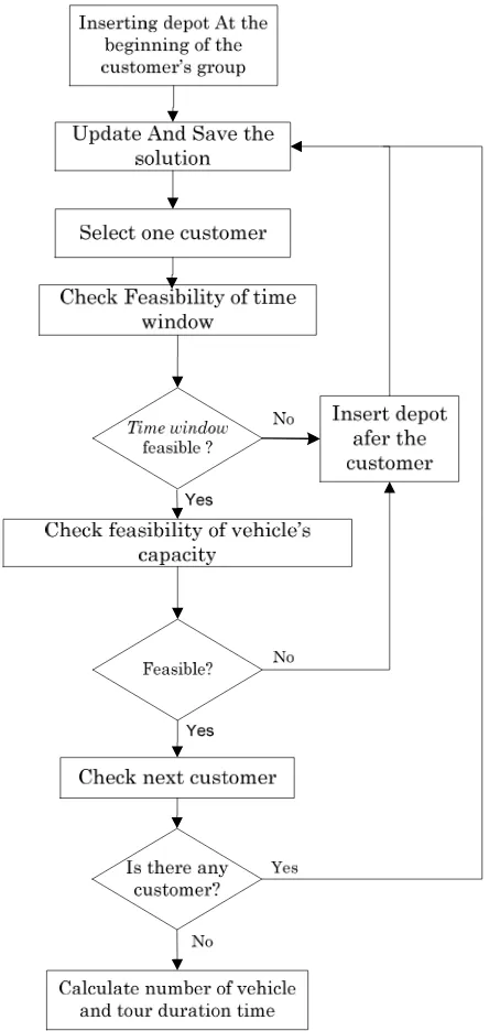
Decoding process is a calculating process to determine number of vehicles based on customer’s time window and vehicle capacity. From the initialization, we will get a sequence of all customers that will be served. Thus, we check the feasible time window and the load constraint for each customer. If it is not feasible, then we add node 0 (depot) after the customer. Flowchart of our decoding process for VRPBMTTW is shown in Figure. 2.
results number of vehicles, total duration tour, and range duration time. From those results, we choose one ant based on objective function that has been predetermined. First priority is number of vehicles. If the first criterion is same from all ants, we choose the second criterion that is the minimum total duration time. So, we do the same thing for the third criterion that is the minimum range of duration time.
Pheromone Update
Pheromone matrix has to be updated in order to make ants choosing the path that is frequently passed. We need total duration time to update the matrix. For the path that has not been passed by ant, we use the following formula:
(40)
Mean while, for the path that has been passed by ant uses the following formula:
(41)
We generate data based on number of backhauls customers and time window. For each data, we use random demand for each customer ranges from 1 to 10 and random distance with coordinate (0,0) to (540,540).We calculate the distance using Euclidean Metric for each customer. A set of data consists of 100 customers whom 50% backhauls customers. The time window varies from tight time window to wide time window. In detail, a tight time window inter-vals ranging from 10 to 50 minutes, while the wide time window ranges from 390 to 540 minutes. We use the mix time window ranging from 10 to 540 minutes and the horizon planning for depot ranges from 0 to 540 minutes.
We used Borland Delphi 2007 and executed on Intel Atom CPU N270 1,6 GHz with 1G DDRAM. Our aim is to find standard parameter settings in order to get good combination of these parameters for VRPBMTTW. Dorigo [8] suggested parameter that express the sensitivity to trace, =1, parameter that states the sensitivity to the desirability, 2 ≤ ≤ 5, and
parameter pheromone trail evaporation, ρ = 0.5 for
travelling salesman problem. From that information, we observed all possibilities to find the combination of these parameters. Finally, we suggested
, 5, and .5.
We analyzed the algorithm performance with 95% confidence level and 10% error. To simplify the analysis, we use equation (1) to compare the results. This equation is totally different if it is compared to
the objective function. There is a contradiction between equation (1) and the objective function. In this case, we want to find the algorithm performance in easy way. So, we use weight for each criterion.
Figure 2 The flowchart of decoding process
Table 1. Experiment results using ACO with z,
, 5, and .5
Experiment Number of Vehicles
Total Tour
Duration Time RDT Z
1 8 2150.65 314.50 1015065
2 9 2070.95 266.10 1107095
3 9 1971.27 306.84 1097127
4 9 2112.67 174.93 1111267
5 7 1406.45 299.16 840645
6 8 2150.65 314.50 1015665
Mean 8.3333 1942.40 272.31 1034239 Standard
Column 5-7 in Table 1 present the results using modified ACO including number of vehicles, total tour duration time, and range of duration time. Column 8 is used to calculate the number of replica-tion by using the following formula:
′ .
. (42)
The result shows that the algorithm has a consistency in solving VRPBMTTW.
We also compare the algorithm to the sequential insertion. The algorithm results better solution to the initial solution. The algorithm provide 8.3 vehicles in average, while the sequential insertion results 10 vehicles.
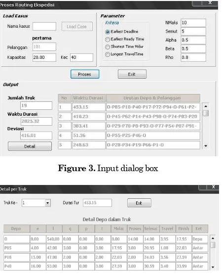
Four rules for selecting the seed customer in the sequential insertion algorithm are provided. These rules are earliest deadline, earliest ready time, shortest time window, and longest travel time. Figure 3 shows four improvement operator arrange-ments are provided.
Figure 4 shows a tour and schedule plan generated using earliest deadline criterion. The tour and schedule plan has information such as sequence of visiting customers, time window, linehauls demand, backhauls demand, arrival and departure time, service time, and travel time.
Figure 3. Input dialog box
Figure 4. An output showing tour and schedule plan
Conclusion
This paper has presented a new variant of the vehicle routing problem with backhauls including the characteristics such as multiple trips, and time windows. The multiple objectives are considered in this paper. An ant colony optimization technique is modified based on the characteristics. The initial feasible solution is generated using sequential insertion with different four seed customer. The computational experiments for others percentage of backhauls should be conducted to show the effectiveness and efficiency of the solution technique including the parameters proposed.
References
1. Bin, Y., Zhong-Zhen, Y., and Baozhen, Y., An
Improved Ant Colony Optimization for Vehicle
Routing Problem. European Journal of
Opera-tional Research 196, 2009, pp. 171–176.
2. Brandao, J. A., New Tabu Search Algorithm for
the Vehicle Routing Problem with Backhauls,
European Journal of Operational Research 173, 2006, pp. 540-555.
3. Bell, J. E., and McMullen, P. R., Ant Colony
Optimization Techniques for the Vehicle Routing
Problem. Advanced Engineering Informatics 18,
2004, pp. 41-48.
4. Bullnheimer, B., Hartl, R. F., and Strauss, C.,
An Improved Ant System Algorithm for the
Vehicle Routing Problem. Annals of Operation
Research 89, 1999, pp. 319-328.
5. Cho, Yuh-Jen., and Wang, Sheng-Der, A
Threshold Accepting Metaheuristics for the Vehicle Routing Problem with Backhauls and
Time Window. Journal of the Eastern Asia
Society for Transportation Studies,6, 2005, pp. 3022-3037.
6. Crispim, J., and Brandao, J., Reactive Tabu
Search and Variable Neighbourhood Descent Applied to the Vehicle Routing Problem with
Backhauls. 4th Metaheuristics International
Con-ference Porto, Portugal July 16-20, 2001.
7. Doerner, K., Gutjahr, W. J., Hartl, R. F.,
Strauss, C., and Stummer, C., Ant Colony Opti-mization in Multiobjective Portofolio Selection,
4th Metaheuristics International Conference,
2001.
8. Dorigo, M., MACS-VRPTW: A Multiple Colony
System for Vehicle Routing Problems With Time
Windows, Ant Colony Optimization,
Massa-chusetts Institute of Technology, London, 1999.
9. Dorigo, M., and Stützle, T., Ant Colony
10. Dorigo, M., and Blum, C., Ant Colony Optimiza-tion Theory: A Survey, Theoretical Computer Science. 344 (2-3), 2005, pp. 243-278.
11. Laporte, G., Gendreau, M., and Potvin, J.,
Classical and Modern Heuristics for the Vehicle
Routing Problem. Transactions in Operational,
2000.
12.Mong Sim, K., and Hong Sun, W., Ant Colony
Optimization for Routing and Load-Balancing:
Survey and New Directions. IEEE Transaction
on Systems, Man, and Cybernetics, 33(5), 2003, pp. 560-567.
13. Suprayogi, and Priyandari, Y., Vehicle Routing
Problem with Multiple Trips, Time Windows, and Simultaneous Delivery and Pickup Services.
Asia Pacific Industrial Engineering and Mana-gement System, 8, 2009, pp. 1543-1552.
14. Suprayogi, Vehicle Routing Problem: Definition,
Variants, and Application. Proceeding Seminar
Nasional Perencanaan Sistem Industri 2003
(SPNS 2003), Bandung, 2003.
15. Tavakkoli-Moghaddam, R., Rabbani, M., Saremi,
A., and Safaei, N., Solving the Backhaul Vehicle
Routing Problem by Genetic Algorithms. 35th
International Conference on Computers and Industrial Engineering, 2005, pp.1905-1910.
16. Zhong, Y., and Cole, M. H., A Vehicle Routing
Problem with Backhauls and Time Window: A
Guided Local Search Solution. Transportation