32 3.1.Methodology of Finite Element Modeling
Modeling started by create geometry model of rough surface and rigid plat. Model of geometry refer to author anylysis regarding topography of real surface. Material defined according to reference from experimental setup [1].
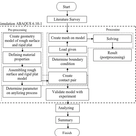
Simulation ABAQUS 6.10-1
Figure 3.1: Flow chart modeling on FEM ABAQUS 6.10-1.
Pre-processing
Create mesh on model Solving
Result (postprocessing)
Determining control type and control solution are really influence on simulation result. Cautious action should be neccesary in order to make the result similar with theory, especilly on determining contact pair (Fig. 3.1).
3.2 Basic Theory of Finite Element Method
The development of the computer world has been so quickly affect the areas of research and industry, so the dream of the experts in developing science and industry has become a reality. Now days, the design and analysis methods have been widely used mathematic complex calculations in many works. Finite element method (FEM) contributed many inventions in the field of manufacture and industry research, this is due to its role as a research tool in numerical simulation.
Finite element method (FEM) is a method of analysis calculations based on the idea of building a very complex object into several simple parts (blocks), or by dividing a very complex object into smaller pieces.
1. The basic concept of FEM analysis.
a. Making the discrete elements to obtain the deviations and forces in smaller scale from the parts of a structure.
b. Using elements of the continuum approach to obtain solutions from the problems of heat transfer, fluid mechanics and solid mechanics. 2. Structure analysis procedures.
a. Dividing the structure into pieces (elements with nodal). b. Providing the physical properties of each element.
c. Connect the elements at each node to form an approximate system of equations for the structure.
d. Solving systems of equations are coupled with an unknown number of nodes (e.g., displacement).
e. Calculate the desired amount (e.g., strains and stresses). 3. Implementations on a computer.
c. Post processing (show results).
4. Types of elements in the finite element method a. One-dimensional elements (lines)
These elements include the type of spring (spring), truss, beam, pipe, etc., as shown in Figure 3.2.
Figure 3.2: Line element.
b. Two-dimensional elements (fields)
These elements include the type of membrane, plate, shell and so on as shown in Figure 3.3.
Figure 3.3: Field element.
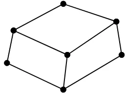
c. Elements of three-dimensional (volume)
These include the element type (3-D Fields-temperature, displacement, stress, flow velocity), as shown in Figure 3.4.
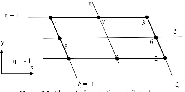
This element is used in two-dimensional problems that require high accuracy in analyzing the model (Fig 3.5).
Figure 3.5: Element of quadratic quadrilateral.
Furthermore,
8
1 1
i Ni (3.2)
Displacement equation (u, v) is
3.3 Specification and Geometry Problem
Authors verify model of surface from present method through applied a particular case of contact elastic deformable rough surface against hard smooth ball (Fig. 3.6.a). In ABAQUS, rough surface model that was imported from SolidWorks is portrayed in Figure 3.6.b the surface for simulation has waviness with multiple heights of asperities. Moreover, surface can easily be meshed with smaller mesh on the top of surface. This particular contact problem will be applied to evaluate the model.
(a) (b)
Figure 3.6: (a) Contact model of rough surface vs hard ball (b) surface geometry in
ABAQUS after being imported from SolidWorks.
There will be three model used in simulation, first is sinusoidal surface, second is random rough surface, and third is experimental model transferred in finite element model. Those models are applied under static contact condition. The software package ABAQUS was used to analyze the three models created in this study.
determine the deformation of various types of contact interactions and compared with each other.
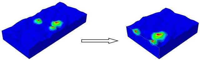
Rough surfaces materials used for all simulations in this study is aluminum. Properties of the material used for experimental data is elastic perfectly plastic with E = 75.2GPa, v = 0.3 and σy = 85.714 Mpa [1] with corresponding material model is frictionless and hard contact. Result from simulation is captured to identify deformed asperity. As cross-sectional pieces surface in which some asperity is deformed as shown in Figure 3.7.
Figure 3.7: Captured surface on cross sectional area.
Modeling using the finite element method which cut surface into several elements (pieces of the surface), then reconnects elements at “nodes” as if nodes were pins or drops of glue that hold elements together. This process results in a set of simultaneous algebraic equations. Each nodes has values which represent condition of surface. Figure 3.8. show the method are used to take values from each nodes. Retrieval results are then plotted in the graph to be displayed in the next chapter.
Mesh densities were increased around the top surface area. The contact load per unit length of the contact corresponding to a given interference was retrieved by summing the reaction forces at each of the nodes in contact with the rigid plane. The contact dimension was obtained from output data files created by the software, which indicated the state of contact at each surface node. Contact pressures and internal stress values were obtained from the standard field outputs of the software. In the finite element simulations described here the term „„interference‟‟ represents the approach of the upper edge of the model towards the contact plane, and zero interference corresponds to initial contact of the undeformed model at zero load. The size of each interference increment was governed by the need to maintain numerical convergence of the iterative solution process embodied in the software to solve the non-linear contact.
3.4 Description of the Modeling Method
3.4.1 Process Pre-processing from Matlab-SolidWorks
3.4.1.1 Determining Surface Geometry on Matlab
Z = h.*randn(N,N);
F = exp(-((X.^2+Y.^2)/(clx^2/2)));
f = 2/sqrt(pi)*rL/N/clx*ifft2(fft2(Z).*fft2(F));
surf(X,Y,f,'FaceColor','interp',...
'EdgeColor','none',...
'FaceLighting','phong')
axis equal off
mg=[f;Y;X]
es=rot90(mg)
sp=reshape(es,[],3)
csvwrite('E:/rough.xyz',sp)
type E:/rough.xyz
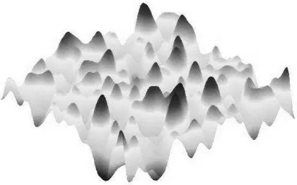
Figure 3.9: Graphic plot of rough surface with n=500, rl=2, h=0.5, and clx=0.2.
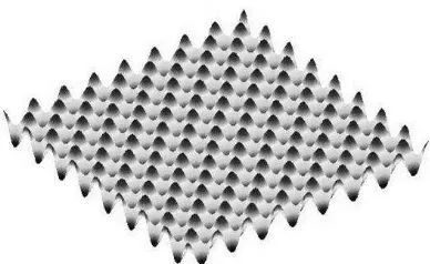
The surface geometry may be changed by modify the script as shown in Figure 3.10 which the surface is designed as sinusoidal surface. Figure 3.10 is using script below:
N=500;
rL=10;
h=0.5;
clx=0.01;
x = linspace(-rL/2,rL/2,N);
y = linspace(-rL/2,rL/2,N);
% Z = h.*randn(N,N);
% F = exp(-((X.^2+Y.^2)/(clx^2/2)));
% f = 2/sqrt(pi)*rL/N/clx*ifft2(fft2(Z).*fft2(F));
f = h.*cos(5.*X).*cos(5.*Y)
surf(X,Y,f,'FaceColor','interp',...
'EdgeColor','none',...
'FaceLighting','phong')
axis equal off
mg=[f;Y;X]
es=rot90(mg)
sp=reshape(es,[],3)
csvwrite('E:/sinusoidal',sp)
type E:/sinusoidal.xyz
Figure 3.10: Sinusoidal rough surface in “xyz” data format.
The generated surface is converted into coordinate surface data. The raw data is exported from the surface data in a triplet or “xyz” data formats which lists the x, y and z coordinate for each point. The triplet information is reformatted so the surface data file becomes a file which creates and fills a 2D surface array.
3.4.1.2 Surface Modification on SolidWorks
At the beginning on SolidWorks, we transformed point cloud into mesh by connecting each nodal to establish rigid geometry of surface. Until this step, the surface was not completely smooth and nearly sharp on each nodal. Therefore, the next step was smoothing the surface with “Scan to 3D” tools in SolidWorks. However, this features only available on “Premium Office” series. This method will generate mesh into solid surface and change its geometry to be perfectly smooth as shown in Figure 3.12.
Figure 3.11: Point cloud file in SolidWorks consisted of numerous nodal as a form of
rough surface with 0.04 pixel size.
(a) (a) (b)
Figure 3.12: Surface which smoothed and given thickness on its surface (a) random
rough surface (b) sinusoidal rough surface.
(initial graphics exchange specification) format data. It is a file format which defines a vendor neutral data format that allows the digital exchange of information among computer-aided design (CAD) systems.
3.4.2 Process pre-processing from ABAQUS
a) Part
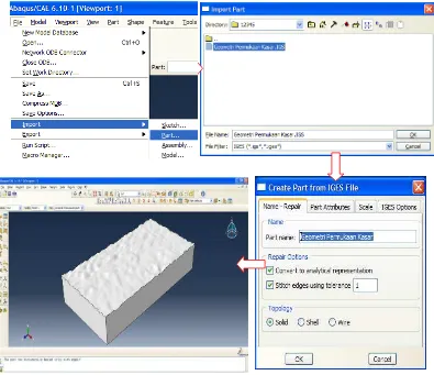
Part geometry is used to create model before simulation. Geometry can be directly made in ABAQUS and can also imported from the CAD software. Rough surface geometry here is obtained from the CAD software format with the extension (*. IGES). Geometry making procedures are shown in Figure 3.13.
Rigid spherical geometry is directly created on ABAQUS. The procedures of making rigid spherical geometry are shown in Figure 3.14.
Figure 3.14: Procedures of making rigid ball geometry.
b) Property
Geometry that has been made on the part is then given material properties. The material used here is elastic-perfectly plastic material with Young's modulus of aluminum E = 75.2 GPa, Poisson's ratio v = 0:34 and the yield stress σy = 85 752 MPa [1]. The material properties when plotted in the form of stress-strain graph shown in Figure 3.15.
Figure 3.15: Graphic of aluminum alloy material properties [1].
Strain ε
[-]
Str
es
s σ
y
(M
P
a)
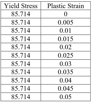
Material properties graphic of aluminum alloy then used in table stress-strain as in Table 3.1.
Table 3.1: Stress-strain of aluminum
Yield Stress Plastic Strain
85.714 0
85.714 0.005
85.714 0.01
85.714 0.015
85.714 0.02
85.714 0.025
85.714 0.03
85.714 0.035
85.714 0.04
85.714 0.045
85.714 0.05
The values of material properties are then submited into software ABAQUS as the procedure in Figure 3.16.
Figure 3.16: Material data input procedures.
not require material properties. Procedures of applying material to geometry are shown in Figure 3.17.
Figure 3.17: Procedures of applying material to geometry rough surface.
c) Assembly
Part geometry at this stage is rough surfaces and spherical geometry rigid. Two geometries are then strung together (assembly) into a screen like the one in the assembly procedure in Figure 3.18.
d) Step
Step procedures is to determine the type of analysis carried out in the ABAQUS software. This type of analysis carried out in this study is a static analysis. Step procedure as in Figure 3.19.
Figure 3.19: Procedures of step.
e) Interaction
Figure 3.20: Procedures of interaction properties.
Click the Create Interaction will appears then click Continue. Select the surface of the ball as the master surface and rough surface as the slave surface.
After edit interaction appears then clicks Create so that Ceate interaction property appears.
f) Load
Load is necessary to determine the loading and boundary conditions (constrain). Load can be a force, pressure, moments and so far depending on the type desired load (Fig 3.21). Boundary conditions can be a displacement, rotation, velocity and so far. As a rigid spherical indenter load is either in the form of interference or contact force at the center of the ball depends desired value. Bottom surface of the rough surface geometry given boundary conditions are not able to move toward any load procedure as in Figure 3.22.
Figure 3.21: Procedures of applying load.
Click so that Create Boundary Condition tab appear, then click Continue, chooses center point of the ball, click done.
Then appear Edit Boundary Condition, select as on picture then click OK.
Click so that Create Boundary Condition will appears, then click Continue, select the lower surface of the rough surface geometry, klik Done.
Figure 3.22: Set-up boundary condition.
g) Mesh
Mesh is to discretize geometry to several elements. Types of elements usedC3D6 (A 6-node linear triangular prism).Mesh procedures as in Figure 3.23.
I. Global seeds.
Entire surface sized 0.1 length /elemen.
Figure 3.23: Sizing control.
II. Local seeds.
Giving the size on rough surface with the length 0.1/elemen (Fig 3.24).
III. Mesh Controls
Select wedge (C3D6) as types of element shape (Fig 3.25).
Figure 3.25: Element shape control.
IV. Mesh part instance
Click to run mesh process then the result as on the picture below (3.26).
Figure 3.26: Surface after being meshed.
h) Job
Figure 3.27: Procedure of job.
i) Visualization
Visualization is used to evaluate the results of the simulation. The results of visualization can be a stress contours and deformation. Results visualization will be shown in chapter four in results and discussion.
3.4.3 Verification of Generated Surface
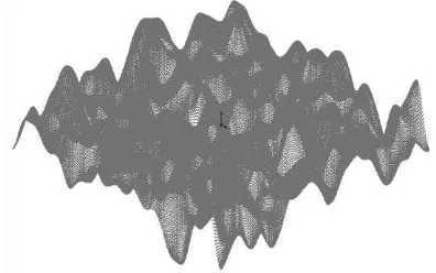
Figure 3.28: (a) Surface generated in form of graphic plot (b) mesh surface after being imported on SolidWorks still has sharp geometry on each nodal (c) half sphere after surface treatment is cut to reduce time computer required (d) surface on ABAQUS.
In the end, the result from those works will be compared to validate present method. In these cases the material properties is considered aluminum (v=0.32; E=70 MPa) with corresponding material model is frictionless. The quarter sphere has 4 mm radius. Contact between the bodies was defined as part of the interaction direction and restrained in the x-direction and the z-direction. The load was defined by applying a constant displacement in the y-direction to the rigid contact plane. This displacement corresponded to the specified interference. For each simulated interference, the model was remeshed to suit the magnitude of deformation expected. These meshed were divided using partitioning tool in the software allowing different meshes of varying element size to be created across the model. Mesh densities were increased around the contact area, and decreased in areas which far from it. An objective in specifying the mesh was to ensure a smooth transition from finely meshed areas to coarser areas thereby avoiding discontinuities in results across partition boundaries within the model.
(b)
ABAQUS and model normally created in ABAQUS are alike. It means further analyzes using present method is justifiable.
Figure 3.29: Comparison between ABAQUS and present model shows good
agreement.
Table 3.2: Comparison of von Misses stress on two models with varying interference
under 433 elements
w S (von Misses) Error %
ABAQUS MSA
0.05 1835 1832 0.163488 0.1 4628 4620 0.172861 0.15 5143 5145 0.03889
0.2 6738 6736 0.029682 0.25 8136 8139 0.03687
0.3 9201 9212 0.11955
Reference:
![Figure 3.15: Graphic of aluminum alloy material properties [1]. [-]](https://thumb-ap.123doks.com/thumbv2/123dok/2244624.1231913/12.595.118.511.179.353/figure-graphic-aluminum-alloy-material-properties.webp)