IDENTIFYING CORRESPONDING SEGMENTS FROM REPEATED SCAN DATA
Bas van Goor, Roderik Lindenbergh and Sylvie Soudarissanane
Dept. of Remote Sensing Delft University of Technology Kluyverweg 1, 2629 HS, Delft, NL
[email protected], [email protected], [email protected], http://enterprise.lr.tudelft.nl/ lindenbergh/
Commission III/3
KEY WORDS:Change detection, LIDAR, point cloud, segmentation, identification
ABSTRACT:
It has been demonstrated that surface changes in the order of millimeters are detectable using terrestrial laser scanning. In practice however, it is still virtually impossible to detect such small changes from for example repeated scans of a complex industrial scene. The three main obstructions are, first, a priori uncertainty on what objects are actually changing, second, errors introduced by registration, and third, difficulties in the identification of identical object parts. In this paper we introduce a method enabling efficient identification that can also be applied to evaluate the quality of a registration. The method starts with a pair of co-registered point clouds, at least partially representing the same scene. First, both point clouds are segmented, according to a suited homogeneity criterion. Based on basically orientation and location, corresponding segment parts are identified, while lack of correspondence leads to the identification of either occlusions or large changes. For the corresponding segments, subtle changes at the millimeter level could be analyzed in a next step. An initial version of the new method is demonstrated on repeated scan data of a metro station experiencing heavy construction works.
1 INTRODUCTION
Detecting changes in scenes sampled by laser scanning data is a topic with a rapidly increasing number of applications, (Vos-selman and Maas, 2010), chapter 7. Administrations, ranging from individual communities to complete countries are initiating airborne laser ranging archives. In The Netherlands for exam-ple, the second version of a nation wide archive is almost com-pleted, while plans have been initiated for a third version, (AHN, 2000). Meanwhile, car based laser mobile mapping systems, (Toth, 2009), are now available in many countries and several researches are initiated to investigate their usage in both built-up, (Haala et al., 2008) and natural environments, (Barber and Mills, 2007). As a consequence, methodology aiming at the detection of changes from such data sources is also under active research, (Champion et al., 2009).
The most easy way to obtain laser point clouds from multiple epochs is by repeatively scanning from a fixed position using a terrestrial laser scanner, e.g. (Little, 2006, Lindenbergh and Pfeifer, 2005). It has been demonstrated, (Gordon and Lichti, 2007), that in a well controlled, close range laser experiment it is possible to measure vertical displacements with an accuracy of ±0.29 mm. To obtain such accuracies from an analysis of re-peated scan data of an arbitrary complex scene is still very chal-lenging however. One major issue is that in general it is on fore-hand unknown what and to what extent objects in the scene were changed.
A computationally efficient method to identify changes is by means of octrees, (Barber et al., 2008, Girardeau-Montaut et al., 2005), that divide the 3D space in small cubical cells, each containing part of the point cloud. Differences in the octree division for different point clouds correspond to changes in the point clouds. Another efficient way is to reduce the 3D problem to 2D by com-paring the relative visibility of different point clouds from one, possibly virtual, viewpoint, (Zeibak and Filin, 2007). By
com-bining the use of octrees with Triangulated Irregular Networks, it becomes possible to analyze changes for individual scan points, (Kang and Lu, 2010).
A disadvantage of these methods is that they are not object ori-ented. An alternative is to first identify objects and in a next step consider if these objects are changed. One way to identify ob-jects in a point cloud is by means of a segmentation method, (Matikainen et al., 2009). In this paper we present a new approach that systematically evaluates segmentations of point clouds of different epochs. The method aims at identifying correspond-ing parts of segments, samplcorrespond-ing the same object. Segments that have no correspondence in other epochs can be linked to occlu-sions or large changes well above the signal to noise ratio. What remains are segments corresponding to the same object surface. In a final step it can be decided using statistical testing methods, whether locally this object surface has changed in a significant way, (Levin and Filin, 2010, Van Gosliga et al., 2006).
2 IDENTIFICATION ALGORITHM
Below we discuss all ingredients of the proposed method in de-tail. We focus on the identification of parts of planar segments that represent the same object.
2.1 Algorithm overview
For convenience we consider here the case of just two point clouds, PC1 and PC2, of approximately the same scene. The method is easily extended in case more point clouds are given. For the mo-ment we also only consider a segmo-mentation into planar segmo-ments. Algorithm 1 summarizes the major steps.
2.2 Registration and Segmentation
Algorithm 1Identifying corresponding segment parts Require: Two point clouds PC1 and PC2 of the same scene.
1: Register PC1 and PC2 in a common coordinate system.
2: Segment both PC1 and PC2 into planar segments.
3: for all resulting segmentsSi do 4: Determine normaln(Si)
5: Determine distanced(Si)from segment plane to origin 6: end for
7: Order segments in PC1 and PC2 according to distancesd(Si) 8: Letnbe the number of segments of PC1
9: Initiate a list CAND ={}of candidate segment pairs
10: for i= 1. . . ndo
11: Take segmentS1
i ∈PC1
16: for all segmentsSin CAND do
17: determine 2D segment polygon△s
18: end for
19: Initiate a list INT ={}of intersecting segment pairs
20: forall segment pairs(si, sj)in CANDdo
26: returnINT, list of segment intersections
are segmented into planar patches, for example using the meth-ods described by (Rabbani et al., 2006). It should be noted that often the segmentation of two different point clouds representing the same scene will lead to different results, even when the same parameter settings are used: Distinct scanners that operated from distinct scan positions will result in point clouds with locally dif-ferent point densities and noise levels. Both point density and noise level will affect the segmentation.
2.3 Segment Plane location
In the following, a first match of segments from both point clouds will be performed, based on two segment properties. These two properties together parameterize the position of the plane con-taining the local planar segment relative to the chosen coordinate system. The first property is the segment orientation, given by the unit normal vectorn = (a, b, c)of the segment. The
sec-ond property is the distance to the origin of the plane containing the segment. LetcS= (cx, cy, cz)denotes the center of gravity
of the points in the segment. The best fitting plane in the least squares sense of the points in the segment passes throughcSand
the distancedSof the plane containingS, to the origin is simply
given as
dS = −a·cx−b·cy−c·cz = −n·cST, (1)
whereT denotes transposition. To increase numerical stability it is convenient to take the center of gravity of, say, the first point cloud as the origin of the local coordinate system.
2.4 Segment Plane matching
The combination of normal vector and distance to the origin are used to determine if two segments, each of one point cloud, are in a common plane, compare Algorithm 1, line 12. A more formal formulation is that the following two conditions should hold for
two segmentsS1
i andS2j from the first and second point cloud
respectively:
|d(Si1)−d(S2j)| ≤ ∆d (2)
6 (n(S1
i),n(Sj2)) ≤ ∆αn, (3)
whered(S1i)andd(Sj2)denote the distance to the origin from
the first and second segment plane, whilen(S1
i)andn(Sj2)
de-note normal vectors of the first and second segments respectively. Here,∆dis a preset distance threshold and∆αna preset
angu-lar threshold, that should be specified by the user, depending on e.g. the quality of the registration and the local noise level of the scan points. The angle6 (u,v)between two vectorsuandvis
computed as
6 (u,v) = arccosu·v (4)
where in addition the two possible antipodal orientations of a nor-mal should be taken into account.
2.5 Reduction to 2D
If for a pair of segments(S1
i, Sj2)both Equation 2 and 3 hold,
both segments are approximately in the same plane but are not necessarily intersecting. They could for example both represent a different part of one big wall. Therefore the area of intersection Sijshould be determined.
△Sij := Si1∩Sj2 (5)
As by now we know thatS1
i and Sj2 are approximately in the
same plane, we can reduce the problem at first approximation to a 2D problem as follows. Letcibe the center of gravity of the
points in segmentS1
i. We consider the projections
s1i = Π(Si1,n1) (6)
s2j = Π(Si2,n1) (7)
of the segmentsS1
i andS2jon the plane throughciperpendicular
to the normal vector of the segmentS1.
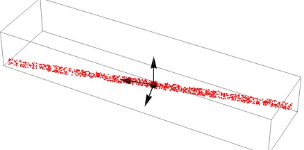
Figure 1: Basis consiting of eigenvectors of the variance covari-ance matrix of the points in a segment.
In practice such projection can be obtained as follows, compare (Lay, 2003). From the centralized segment
S1i := Si1−Ci1, (8)
withC1
i the matrix with each row equal to the center of gravity
of the points in segmentS1
i, the eigen vector matrixEi1of the
variance-covariance matrix ofS1i is determined:
Ei1 := eigen vectors(S
1
i) T
·S1i (9)
in segmentS1
i, the second eigen vector in the remaining
orthogo-nal direction of maximal variation, while the last points in the re-maining orthogonal direction that has least variation, see also Fig-ure 1. As a consequence, the first two eigen vectors span (in most cases) the least squares plane through the (centralized) points of segmentS1
i. Therefore the desired projection is obtained by
ex-pressing the (centralized) segment points of both segments with respect to this eigenvector basis for the first, reference segemnt:
˜
In this new coordinate system, the first two coordinates express the location of a point in the segment plane ofS1
i, while the third
coordinate gives the distance of the point to the plane.
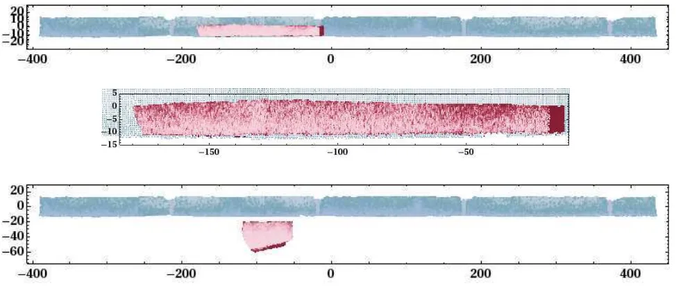
In Figure 2 the results of such projection are illustrated.
2.6 2D Segment intersection
What remains, see also Figure 2, is to find the intersection of two planar segmentss1
i ands2j. To increase efficiency, this is done
in two steps. First, for both segmentss1
i and s2j, the bounding
are determined, where e.g.xm
i denotes the minimalx-coordinate
of the points in segments1
i andy M
j the maximal y-coordinate
of the points in segments2
j. If the bounding rectangular boxes
for both segments do not intersect, the segments themselves cer-tainly do not intersect. If the bounding boxes do intersect, the second step only has to consider the points of both segments in the intersection.
In the second step the points from each segment (in the intersec-tion) are organized in a raster, with a preset width, of, say, 5 cm. If a raster cell contains a segment point, it is given the value1, otherwise it gets the value0. The intersection of both segments is now determined from overlaying the two rasters. Only if two corresponding raster cells both have the value1, it belongs to the intersection of the two segments. This method is flexible in the sense that it also deals with segments with holes, corresponding e.g. to a window in a door.
This method can be further refined by using quad-trees instead of simple rasters: the quad-tree structure can be used to more precisely define the boundary of the segments. Each raster cell containing segment points, but 4-adjacent to an empty raster cell, is subdivided into four smaller cells, until a minimal cell size is reached. The intersection of two such quad-trees, each corre-sponding to a segment, basically works the same as intersecting two rasters.
2.7 Implementation
The described method is relatively easy to implement. Using least squares adjustment, (Teunissen, 2000), the normal of each segment can be derived. The same least squares adjustment can be used to project candidate corresponding segments to the least squares plane of the first segment. What remains is construct-ing a raster or quad-tree for a relative small number of possibly intersecting segment parts
3 RESULTS AND DISCUSSION
In this section, the potential of the method described in Section 2 is illustrated for a case study. It should be noted however that
the method used to obtain the results below was an initial method that differences at details from the method described in Section 2.
3.1 Data description
For the case study we consider two point clouds representing a part of the Rotterdam Central metro station. The selected area covers an area of 8×3 m of the wall on the southern side of the tunnel, see Figure 3. During the first epoch, acquired at April 24, 2006, approximately 350 thousand points of this specific part of the tunnel were sampled from one standpoint using the Z+F Imager 5003 phase based scanner. During the third epoch, d.d. November 20, 2007, 3.5 million points were obtained, from two different standpoints, compare also Figure 3, left, using the Faro LS880 phase based scanner. From one of these standpoints, two scans were acquired, resulting in three available scans in this epoch.
Registration of individual scans was performed using the soft-ware Cyclone from Leica. Both control points and object match-ing were used. In Epoch 1, the reported accuracy was 3 mm, in Epoch 3, it was 6 mm. Control points were additionally measured with a total station, and both point clouds were georeferenced to the same absolute coordinate system RDNAP. The two resulting point clouds are shown in Figure 4. The effect of grafitti on the in-tensity measurements is clearly visible in both epochs. In Epoch 3, on the right, the footbridge is visible, indicated by a red ellipse, which was not yet present in Epoch 1.
3.2 Segmentation
Point clouds from both scans were segmented into planar patches using the region growing method described in (Rabbani et al., 2006). The method requires three parameters, a number,k, of neighbors for each point, an angular threshold,αp, to compare
local surface normals, and a distance threshold,dp, that considers
the distance between the point at hand and a growing segment. Here, the parameter valuesk = 30,αp= 30◦anddp =.03m
were used. These setting resulted in 20 segments for Epoch 1, and 494 segments for Epoch 3. The increase in the number of segments from Epoch 1 to Epoch 3 already indicates that more different objects are in the scene in Epoch 3.
3.3 Corresponding segments
For deciding if two segments from two different epochs intersect, some additional parameter values have to be set, as described in detail in Section 2.3. First, it is decided if two segments are in the same plane. For this purpose, the maximal difference,αS, in
orientation between two segments is set at10◦
. Moreover, the distance,dS, between segments, as defined in Section 2.3, should
not be more than 0.10 m. To determine if two segments in the same plane intersect, no additional parameters were needed.
Figure 2:Top:Two intersecting segments, with blue and red points resp. , in a common segment plane;Middle:Same, but zoomed in on the red points;Right:Two non-intersecting segments in the same segment plane. Axes are labeled in centimeter.
3.4 Possible large changes
Points that have no correspondence are shown in Figure 6. Points that are marked by a capital ‘A‘ are located at the edges of the data sets and have no correspondence because the two data sets were cropped in a slightly different way; Points marked by ‘B‘ are situated behind the location where later the footbridge would be placed in Epoch 1, and on the footbridge in Epoch 3. Similarly, points marked ‘C‘ correspond to points behind and on water pipes that were added to the scene between epochs.
3.5 Possible changes in intersecting segments
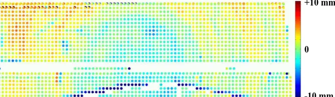
Figure 7 illustrates the distances between points from correspond-ing segment parts. The method proposed in this paper allows to efficiently identify such correspondences. Still very interesting differences may occur between points from corresponding seg-ments. A first type of differences may be caused by registration errors. Errors caused by registration are expected to be locally stable, that is, for a point cloud covering several tenths of meters, the registration error between two point clouds is expected to be more or less the same over a stretch of one meter.
To mitigate the effect of registration errors, the mean difference between points belonging to corresponding segments can be re-moved, which is how Figure 7 is obtained. What remains are differences that can be caused by either real local differences in the surface elevation or by local scanner artifacts. In Figure 7, a circular pattern is visible corresponding to some systematic dif-ferences in the order of a few millimeter.
There are two possible explanations for this particular pattern. The first is hardware related. In Figure 3 it can be seen that in both cases the scanner was located directly in front of the region of interest. This may have resulted in some saturation effect that could explain the circular pattern. Another possible explanation is physical. The signal may be the result of ground water outside the tunnel. The footbridge is placed at this location to protect a water inlet. Below the footbridge, a water tap is constructed to inject water in the ground around the tunnel. The water tap is connected to the water pipes that run through the tunnel. The
ground around the tunnel presses on the exterior of the tunnel. When the water is injected in the ground, the pressure on the tunnel increases. The increase is the largest around the injection point, below the footbridge. Further away the pressure decreases, which may explain the circular pattern.
4 CONCLUSIONS AND FUTURE WORK
In this paper a new method has been presented that in an effi-cient way identifies corresponding parts of different point clouds representing the same planar feature. This method allows to de-compose repeated point clouds in components corresponding to large changes or occlusions on one hand and components sam-pling the same object surface on the other hand. The method is computationally efficient, given a segmentation into planar seg-ments. The method can be extended to segmentations including other geometric shapes, like cylinders or spheres. As a conse-quence it would be suitable for analyzing repeated point clouds of most human made objects. In combination with the methods of e.g. (Zeibak and Filin, 2007) a complete work flow can be obtained considering both possible changes close to the signal to noise ratio, occlusions and large changes.
ACKNOWLEDGEMENTS
Figure 3: Left: Schematic representation of scanner standpoints in both epochs and area of interest. Right: Photograph of the footbridge taken in January 2010.
high
low
high
low
Figure 4: Relative intensities.Left.Epoch 1.RightEpoch 3. The location of the footbridge is indicated by a red ellipse.
Figure 5: Corresponding Segments.Left:Epoch 1.RightEpoch 3. Correspondences are indicated by color.
Figure 6: Possible changesLeft:Epoch 1.RightEpoch 3.
+10 mm
0
REFERENCES
AHN, 2000. Productspecificaties AHN1 en AHN2. Technical re-port, Rijkswaterstaat, DID. http://www.ahn.nl, last visited: June 26, 2011.
Barber, D. and Mills, J., 2007. Vehicle based waveform laser scanning in a coastal environment. In: Proceedings 5th Inter-national Symposium on Mobile Mapping Technologies, Padua, Italy.
Barber, D., Holland, D. and Mills, L., 2008. Change detection for topographic mapping using three-dimensional data structures. IASPRS XXXVII(B4), pp. 1177–1182.
Champion, N., Rottensteiner, F., Matikainen, L., Liang, X., Hyypp¨a, J. and Olsen, B. P., 2009. A test of automatic build-ing change detection approaches. International Archives of Pho-togrammetry, Remote Sensing and Spatial Information Sciences XXXVIII(3/W4), pp. 145–150.
Girardeau-Montaut, D., Roux, M., Marc, R. and Thibault, G., 2005. Change detection on points cloud data acquired with a ground laser scanner. In: Proceedings ‘Laser scanning 2005’, Enschede, The Netherlands.
Gordon, S. J. and Lichti, D. D., 2007. Modeling terrestrial laser scanner data for precise structural deformation measure-ment. Journal of Surveying Engineering 133, pp. 72–80.
Haala, N., Peter, M., Cefalu, A. and Kremer, J., 2008. Mobile lidar mapping for urban data capture. In: Proceedings 14th Inter-national Conference on Virtual Systems and Multimedia, pp. 95– 100.
Kang, Z. and Lu, Z., 2010. The change detection of building models using epochs of terrestrial point clouds. International Archives of Photogrammetry, Remote Sensing and Spatial Infor-mation Science XXXVIII(8), pp. 231–236.
Lay, D. C., 2003. Linear Algebra. third edn, Addison Wesley.
Levin, S. and Filin, S., 2010. Archeological site documentation and monitoring of changes using surface-based photogrammetry. International Archives of the Photogrammetry, Remote Sensing and Spatial Information Sciences XXXVIII(5), pp. 381–386.
Lindenbergh, R. and Pfeifer, N., 2005. A statistical deforma-tion analysis of two epochs of terrestrial laser data of a lock. In: Proceedings 7th conference on optical 3-D Measurement Tech-niques, Vienna, Austria.
Little, M., 2006. Slope monitoring strategy at PPRust open pit operation. In: Proceedings International Symposium on Stability of Rock Slopes in Open Pit Mining and Civil Engineering, Megan Little, South Africa.
Matikainen, L., Hyypp¨a, J., Ahokas, E., Markelin, L. and Kaarti-nen, H., 2009. An improved approach for automatic detec-tion of changes in buildings. International Archives of Pho-togrammetry, Remote Sensing and Spatial Information Sciences XXXVIII(3/W8), pp. 61–67.
Rabbani, T., Van den Heuvel, F. and Vosselman, G., 2006. Seg-mentation of point clouds using smoothness constraints. IASPRS XXXVI(5), pp. 248–253.
Teunissen, P. J. G., 2000. Adjustment theory. Delft University Press, Delft.
Toth, C., 2009. R&D of Mobile Mapping and future trends. In: Proceedings of the ASPRS Annual Conference, Baltimore, United States.
Van Gosliga, R., Lindenbergh, R. and Pfeifer, N., 2006. Defor-mation analysis of a bored tunnel by means of terrestrial laser scanning. IASPRS XXXVI(5), pp. 167–172.
Vosselman, G. and Maas, H.-G. (eds), 2010. Airborne and Terres-trial Laser Scanning. Whittles Publishing, Dunbeath, Scotland, chapter Engineering Applications, pp. 237–269.