Conference paper

(1)

EMULATION OF LISS III IMAGES FOR HIGH TEMPORAL RESOLUTION AT LARGER

SWATH

C.V.Rao a, *, J. Malleswara rao a, A.Senthil Kumar a, B.Lakshmi a , V.K. Dadhwal a

a

National Remote Sensing Centre, Indian Space Research Organization, Hyderabad 50037, India rao_cv@nrsc.gov.in

KEY WORDS: Spatio-temporal Data Fusion, Swath Expansion, Single-Image-Super resolution, AWiFS and LISS III sensors Data

ABSTRACT:

Space borne sensors have limited capability to acquire images at high spatial and high temporal resolutions with larger swath simultaneously. In this paper, we propose alternatives to overcome this limitation by emulating such images at ground data processing system. Resourcesat-2, one of the Indian Space Research Organization’s (ISRO) mission carries Linear Imaging Self-Scanners (LISS III and LISS-IV) and an Advanced Wide-Field Sensor (AWiFS) onboard. The spatial and temporal resolutions of LISS III are 23.5 m and 24 days, and those of AWiFS are 56 m and 5 days, respectively. The 141 km swath of LISS III data is overlapped with the 740 km swath of AWiFS data at centre portion in simultaneous acquisition. Two novel approaches are proposed to emulate the LISS III image with 740 km swath at 23.5 m spatial and 5-days temporal resolutions. First approach is to emulate the synthetic LISS III images at 23.5 m spatial and 5-days temporal resolutions. Mosaic such images to cover the full 740 km swath of AWiFS for a given date. First approach is achieved through a spatio-temporal data fusion technique which depends on the previously acquired single AWiFS-LISS III image pair. Second approach assumes that the non-overlapping region of AWiFS contains similar Earth’s surface features of LISS III overlapping region; then it is possible to enhance the spatial resolution of AWiFS to the spatial resolution of LISS III in the non-overlapping region. It is achieved through a single-image-super resolution technique over Non-sub sampled Contourlet Transform. First approach is computationally efficient but it requires prior knowledge of a single AWiFS-LISS III image pair for each emulated LISS III image. That image pair is acquired before or after the prediction date. Also, first approach faces radiometric issues in the mosaic process. Second approach has high computational complexity. But it works well for the data sets which are satisfying the above basic assumption. An accuracy of both methods is validated with originally acquired LISS III data sets. Experimental results demonstrated that the accuracy of first approach is around 92% and the second approach is around 87%. In the second approach, only the overlapping regions of AWiFS and LISS III in simultaneous acquisition are used as prior knowledge. The accuracy of this method can be improved by increasing the database of the relevant prior knowledge.

* Corresponding author. rao_cv@nrsc.gov.in

(2)

1. INTRODUCTION

The Earth Observation (EO) satellites images are used to map and monitor the natural resources. The map precision increases with an increase in the capabilities of remote sensing (RS) sensors technology. High spatial resolution improves the accuracy of the thematic maps (Mumby and Edwards 2002). If spectrally heterogeneous classes contain fine spatial resolution data, classification accuracy will be increased (Lillesand and Kiefer 1994). The high temporal resolution data is used to monitor the biodynamic nature of the Earth’s surface features (Hilker et al. 2009). There is a trade-off between high spatial and high temporal resolutions in designing the space borne sensor. It is either necessary to find a compromise between the spatial and temporal resolution according to the requirement of an application or to utilize an alternative method of data acquisition.

Data fusion combines the information from multiple sensors to make inferences which are not possible with a single sensor (Hall and McMullen 1992). Image fusion combines the data synergistically from different sensors to achieve the best information (Pohl and Van Genderen 1998). Therefore, multiple applications are depending on the multi sensor data fusion to derive and analyze the information (Rao et al. 2014c).

Image-super-resolution constructs the high-spatial resolution image by combining the sequence of low-spatial-resolution images which are having sub-pixel shifts (Joshi et al. 2004). But single-image-super resolution image learns the spatial-resolution image from the training database of low and high-spatial-resolution image patches for a given low-spatial resolution image (Gajjar et al. 2010).

The main objective of the current study is to create a synthetic LISS III image at 23.5 m spatial and 5-days temporal resolutions at 740 km swath. In this paper, we achieve the objective with spatio-temporal image fusion and single-image-super-resolution techniques developed by Rao et al. (2014a, 2014b).

2. BACKGROUND

2.1 Spatio-temporal Image Fusion

Generally spatial-spectral fusion methods are traditionally in use. Spatial-spectral fusion methods improve the spatial resolution of low resolution multispectral image while preserving the spectral information. In contrast, spatio-temporal fusion method improves repetitiveness of LISS III images, and the resultant pixel values estimated for better temporal resolutions simultaneously while retaining all other characteristics

Gao et al. (2006) uses MODIS and Landsat images in Spatial and Temporal Adaptive Reflectance Fusion Model (STARFM). This method predicts the synthetic Landsat image at MODIS temporal resolution and it uses one or two input pairs of MODIS-Landsat images as prior knowledge. Hilker et al. (2009a) analyzed the potentiality of STARFM and generated synthetic Landsat images at MODIS temporal resolution. Hilker et al. (2009b) proposed a Spatial and Temporal Adaptive Algorithm for mapping Reflectance Change (STAARCH) which reconstructs the changes in land cover with the help of Tasseled Cap transformations of both Landsat and MODIS reflectance data. The STARFM and STAARCH methods face difficulty in detecting and delineating the land-cover-type changes in synthetic Landsat imagery (Huang and Song 2012).

Sparse representation based Spatial Temporal Reflectance Fusion Model (SPSTFM) has developed recently which uses two input pairs of MODIS-Landsat images as prior knowledge (Huang and Song 2012). This method establishes a correspondence between structures within high spatial resolution (HSR) image and their corresponding low spatial resolution (LSR) image using sparse representation. Song and Huang (2013) developed a spatiotemporal data fusion based on the dictionary learning (DL) with one input pair of MODIS-Landsat images. The results show a better performance in comparison with STARFM method. computationally efficient spatiotemporal data fusion method in operation mode for larger study areas. In this paper, we demonstrated the effect of computationally efficient spatio-temporal image fusion method of Rao et al. (2014a) for AWiFS and LISS III sensor images.

2.2 Non-sub-sampled contourlet transform (NSCT)

Do and Vetterli (2005) proposed contourlet transform (CT) to represent two dimensional singularities of an image. The CT composed with Laplacian pyramid (LP) and directional filter bank (DFB). Although CT transform represents curves sparsely due to its directionality and anisotropy, there is a frequency aliasing in the process of decomposition and reconstruction of an image in the CT. To reduce the frequency aliasing, enhance directional selectivity and shift-invariance, Cunha et al. (2006) proposed Non-Sub-sampled Contourlet Transform (NSCT) based on sampled pyramid decomposition and non-sub-sampled filter banks (NSFB). NSCT is the shift-invariant version of CT. NSCT uses iterated non-separable two-channel NSFB to obtain the shift-invariance and to avoid pseudo-Gibbs phenomena around singularities.

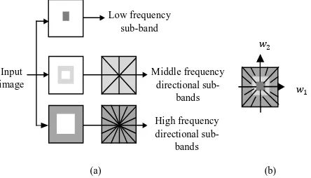
The NSCT not only provides multi-resolution analysis, but also contains geometric and directional representation. Figure 1 shows the overview of the NSCT and Figure 1(a) shows non sub sampled filter banks structure. The NSCT structure is composed of a filter banks which split the 2-D frequency plane into sub bands. Frequency partitioning is illustrated in Figure 1(b). NSCT get the perfect reconstruction through reconstructing filter banks. NSCT is more efficient than other multi-resolution analysis in image de-noising and image enhancement due to its multi-scale, multi-direction, anisotropy and shift-invariance (Cunha et al. 2006). Therefore, we perform multi-resolution decomposition on remote sensing images by NSCT to enhance the spatial resolution through Contourlet Coefficients Learning (CCL).

(b) (a)

Figure 1. Nonsubsampled contourlet transform, (a) Non sub sampled filter banks structure that implements the NSCT, (b) Frequencuy partitioning obtained with the filter banks shown in (a) .

Input

(3)

2.3 Support Vector Regression (SVR)

The support vector machines (SVM), originally proposed as a learning algorithm with the ability to provide function estimation (Chang and Lin. 2011). By using a mapping, ∶ → ℱ, where is the domain and ℱ is usually a high-dimensional feature space, support vector regression (SVR) work in feature space to approximate unknown functions in an output space. And then non linear functions are used to linearly estimate an unknown regression.

Suppose that we have a training set with input-output pairs as in (1)

The objective of Super-Resolution (SR) methods is to recover a high resolution image from one or more low resolution images (Rao et al. 2011). SR methods are broadly classified into two types (i) the classical multi-image super-resolution, and (ii) single-image super-resolution. In the classical multi-image SR a set of low-resolution images of the same scene are taken at sub-pixel shifts. Each low resolution image imposes a set of linear constraints on the unknown high resolution intensity values. If sufficient number of low-resolution images is available at sub pixel shifts, the set of equations can be solved to recover the high-resolution image. This approach is numerically limited only to small increases in the spatial resolution.

In a single-image SR, correspondences between low and high resolution image patches are learned from a database of low and high resolution image pairs (usually with a relative scale factor of 2). The learned image patches are used to recover its most probable high-resolution version for a given new low-resolution image. In a single-image SR, missing high-resolution information is assumed to be available in the high-resolution database patches, and learned from the low-resolution and high-resolution pairs of examples in the database. In this paper we demonstrated the single-image-super resolution for swath expansion through the NSCT and an SVR.

3. METHODOLOGY modulating the derived high frequency details from previously AWiFS-LISS III image pair at time as shown in Equation (5)

= + 4∗ ( , , )− ( , , ) ∗ ( 5)

To cover the full 740 km swath for a particular date, we have to mosaic 25 LISS III scenes approximately as shown in Figure 2.

Figure 2. Full AWiFS scene approximately covered by the 25 LISS III images which are acquired in different dates

For example, an AWiFS image is acquired on 11-3-2014 in the path 93 row 52 at 740 km swath. In simultaneous acquisition, LISS III image on 11-3-2014 is also acquired at 141 km swath in the same path and row at the centre portion of the full AWiFS scene as shown in Figure 2.To create a synthetic LISS III image at 740 km swath for 11-3-2014; we need to emulate other LISS III images for 11-3-2014. The International Archives of the Photogrammetry, Remote Sensing and Spatial Information Sciences, Volume XL-8, 2014

(4)

The proposed spatio-temporal data fusion requires previously acquired single AWiFS-LISS III image pair as prior knowledge. In path 91, LISS III images are acquired on 1-3-2014, but we require these LISS III images for 11-3-2014. Originally, in this path, there is no LISSS acquisition on 11-3-2014. In this work, we emulated the LISS III images for 11-3-2014 in the path 91 by using a AWiFS image on 11-3-2014 in that path and previously acquired single AWiFS-LISS III image pair on 1-3-2014 in that path. Therefore, we can predict similarly for the other paths 92, 94, 95. Here LISS III image in the path 93 is originally acquired on 11-3-2014. Hence the all the LISS IIII images in paths 91, 92, 93, 94 and 95 are emulated for the date 11-3-2014. Mosaicking of all such images forms a synthetic LISS III image at 740 km swath.

3.2 Creation of HSHT Images at a wider swath through Single-Image-Super Resolution

Figure 3. Overlapping and non-overlapping regions of AWiFS and LISS III images in a simultaneous acquisition. Light gray colour represents the non-overlapping region and dark gray colour rectangle represents the overlapping region.

The main objective is to enhance the spatial resolution of AWiFS image to the spatial resolution of LISS III image in the non-overlapping region. Consequently the swath of LISS III image expands to the swath of AWiFS image. Assume that the non-overlapping region AWiFS contains the similar Earth’s surface features of LISS III overlapping region. Then it is possible to enhance the spatial resolution of AWiFS to the spatial resolution of LISS III in the non-overlapping region. With this assumption, in this paper, we demonstrated the swath expansion with single-image–super resolution technique through the NSCT and an SVR.

3.2.1 Single-Image-Super Resolution through NSCT

3.2.1.1

Training Phase

An AWiFS image is rectified to maintain the identical geometry of LISS III image through the process of the geometric correction. Consequently, pixels in the overlapping region of AWiFS and LISS III images are in one-to-one correspondence. Training data for each sub band was created by applying the Non-Sub sampled Contourlet Transform (NSCT) to the overlapped LISS III and its corresponding interpolated AWiFS image.

(a). Extract the sub scene of AWiFS image corresponding to the overlapped LISS III from the full AWiFS scene.

(b). Apply the NSCT to the overlapped LISS III and its corresponding AWiFS image. The 2-level decomposition was applied in the NSCT. Middle level frequencies were decomposed into two directions and high level frequencies

were decomposed into four directions. The remaining frequencies were in low-pass sub-band.

(c). Extract 5 × 5 patches with 5 × 5 moving window, this window moves towards right side by one column. After end of the columns, it moves down by one row. Repeat the same procedure until to cover the whole sub band. The training data was created for each sub band in each level and direction

Each row in training data contains pixels of 5 × 5 LISS III patch and its corresponding pixels of 5×5 AWiFS patch of the

Interpolated full AWiFS image contains both overlapping and non-overlapping regions. The interpolated full AWiFS image is taken as input image to enhance the spatial resolution of the non-overlapping.

(a) Apply NSCT to the interpolated full AWiFS scene. The number of levels and directions are same as in training phase. (b) Extract a 5 × 5 patch from a sub band. Identify the best

matched 5 × 5 AWiFS sub band patch in the training data where the root mean squared error is minimum between the given 5 × 5 AWiFS patch and all 5 × 5 AWiFS patches in the training data.

(c) The corresponding 5 × 5 LISS III patch of the best matched 5 × 5 AWiFS patch is the desired 5 × 5 LISS III patch. Move this 5 × 5 window with one pixel overlap and repeat the same procedure until to cover the whole sub band. An average was taken between the pixels of one pixel overlap. (d) Apply inverse NSCT to the predicted sub bands. The HR

LISS III image is created for both the overlapping and overlapping regions. Hence the spatial resolution of non-overlapping region is enhanced to the spatial resolution of The SVR prediction output corresponding to this input vector is a LISS III pixel at location I. The overlapping regions of the simulated AWiFS image and the LISS III image were used to create the training data. In prediction step of the SVR method, for a given AWiFS pixel at location J, neighbourhood window of 5×5 is used to create the input vector. For this input vector, 100 best training sample were selected from the training data. An SVR model was trained with these 100 training samples. The trained SVR model was used to predict the LISS III pixel at location J for a given AWiFS pixel at location J. We have trained the SVR model with the same set of parameters for the whole image. Radial basis function was used as the kernel function. A grid-search was performed to optimize the kernel parameters gamma and the cost of constraint constant. The grid-search resulted in values of 10 for gamma and 50 for the cost. The epsilon value is set as 0.1. However, an SVR model is a data driven method, different data sets may have different parameter settings. In our experiments, we have developed an SVR super resolution tool with MATLAB using a library for support vector machines (LibSVM) (Chang and Lin. 2011).

(5)

4. EXPERIMENTAL RESULTS AND ANALYSIS

4.1 Results of spatio-temporal image fusion approach We consider the original LISS III data along the centre path of the AWiFS full scene i.e. 93 path as shown in the Figure 2. The remaining paths 91 and 92 on the left side, the 94 and 95 paths on the right side of the centre path 93 were considered to predict LISS III images for 11-3-2014.

Along the path 93, LISS III data is acquired on 11-3-2014, but the data in the preceding path 92 is acquired on 6-3-2014. For the path 92, we have AWIFS-LISS III image pair acquired on 6-3-2014 and an AWiFS image acquired on 11-3-6-3-2014. By using these data sets, we predicted the LISS III image for 11-3-204 in the path 92. Therefore, now in 92 and 93 paths, we have LISS III images for 11-3-2014. To cross-validate the predicted image in the path 92 for the 11-3-2014, we have an opportunity to use the overlapping region between the paths. Here 93 path LISS III image is originally acquired image. But 92 path LISS III image is predicted image. These two images have 20 to 30% overlap. Figure 4 shows the 70 km swath strips in 92 and 93 path. The yellow colour polygon is the overlapping region between the two images. We have tested the accuracy of the overlapping region for predicted LISS III image with the original LISS III image. Quantitative results are shown in Table 1.

Spatial quality of the predicted images were evaluated with the root mean squared error (RMSE) and structural similarity index map (SSIM) (Wang et al. 2004). Spectral quality is evaluated with the spectral angle mapper (SAM). An average RMSE of four bands is 0.0093 in reflectance values. The SAM value is 2.785 in degrees. The SSIM provides the local structural information of an image. An average SSIM of the four bands is 0.89. The prediction accuracy is evaluated with the statistical parameter . The prediction accuracy for each band is shown in Figure 5. An average of four bands is 0. 92 i.e. the prediction accuracy of the spatio-temporal data fusion approach is 92% for this experimental data set.

Figure 4. (a) Orignal LISS III image on 11-3-2014 along the path 93 and predicted LISS III for 11-3-2014 along the path 92.The yellow color polygon is the overalpping region, (b) zoomed original LISS III image , (c) zoomed predicted LISS III image of black colour box in the yellow colour polygon.

Table 1. Quantitative results of the spatio-temporal data fusion approach

Figure 5. Scatter plots of the original LISS III reflectance values against the predicted LISS III reflectance values for each band (where scale factor is 1000).

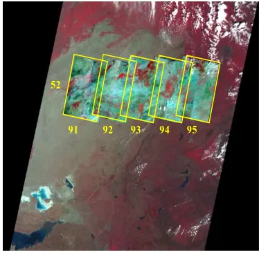
In a similar manner, we can predict LISS III images for 11-3-2014 in other paths 91, 94 and 95 also. The predicted LISS III images for the row 52 in paths 91 to 95 are shown in Figure 6. By predicting LISS III images for 11-3-2014 in other rows, we can obtain an emulated LISS III image at 740 km swath at AWiFS revisit cycles.

Figure 6. Predicted LISS III images for 11-3-2014 along the path 91, 92, 94 and 95 in the row 52 overlaid on the full AWiFS scene. The image in the path 93 is the original LISS III image of 11-3-2014.

B2 B3 B4 B5

RMSE(reflectance) 0.0072 0.0111 0.0085 0.0107

SSIM 0.9232 0.9510 0.8745 0.8512

(a)

(b)

(c)

93 92

91 94 95

52

Quality parameter

Bands

(a) _(b)

(c) _(d)

(6)

4.2 Results of single-image-super-resolution through NSCT

We evaluated the effect of the proposed method on the spatial resolution difference only. We created a simulated AWiFS image by degrading the LISS III image of size 300 × 300. Then the size of the simulated AWiFS image is 300 × 300. A sub scene of 150× 150 image at the centre of 300 × 300LISS III image was used as overlapped LISS III on the simulated AWiFS image. Therefore the simulated AWiFS and the centre 150 × 150 LISS III image have no radiometric, geometric, spectral and bi-directional reflectance distribution function (BRDF) differences. They have only the spatial resolution difference. The overlapping 150 × 150 regions of LISS III and AWiFS are used for training. The non-overlapping-region of AWiFS is used for testing.

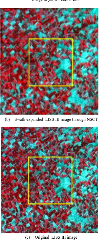
Figure 8(a) is the simulated AWiFS image with overlapped LISS III image in yellow colour box, Figure 8(b) is the swath expanded LISS III using CCL and Figure 8(c) is the original LISS III image. Quantitative results are shown in Table 2. An average RMSE of four bands is 0.0069 in reflectance values. The SAM value is 2.541 in degrees. The SSIM provides the local structural information of an image. An average SSIM of the four bands is 0.91. The prediction accuracy is evaluated with the statistical parameter . The prediction accuracy for each band is shown in Figure 7. An average of four bands is 0. 92 i.e. the prediction accuracy of the single-super-resolution approach through NSCT for the simulated data sets is 92%.

Table 2. Quantitative results of single-image-super resolution approach through the NSCT.

Figure 8. Enhancement of AWiFS spatial resolution to the spatial resolution of LISS III in the non-overlapping region by the CCL.

B2 B3 B4 B5

RMSE (reflectance) 0.0040 0.0084 0.0085 0.0070

SSIM 0.9102 0.9256 0.8941 0.9152

Bands Quality

parameter

(a) (b)

(c) (d)

(a) Simulated AWiFS scene with overlapped LISS III image in yellow colour box

(b) Swath expanded LISS III image through NSCT

(c) Original LISS III image

(7)

In practical, the input data sets contain geometric, radiometric, spectral and BRDF differences between AWiFS and LISS III images. The Counterlet Coefficients Learning (CCL) method works well for the data sets which do not have these differences. The CCL method follows the shift invariance property of the NSCT in multi-scale decomposition. If there is any small geometric bias between AWiFS and LISS images, the CCL method faces the difficulty in learning the correspondence between the AWiFS and LISS image patches in the overlapping regions. For real data sets of AWiFS and LISS III images an alternative methods are required.

4.3 Results of single-image-super-resolution through SVR Support vector regression is a data driven method to predict the unknown data with a prior knowledge. It predicts the high resolution data in pixel-wise. So that it takes high computational time to train the database of high resolution pixels and its corresponding low-resolution patches. However, our experimental results demonstrated that SVR predicts appropriately for real AWiFS and LISS III data sets. It has been observed that SVR predicts proper high resolution pixels for a given low-resolution patches even for the sub-pixel geometric bias in the overlapping region of AWiFS and LISS III images.

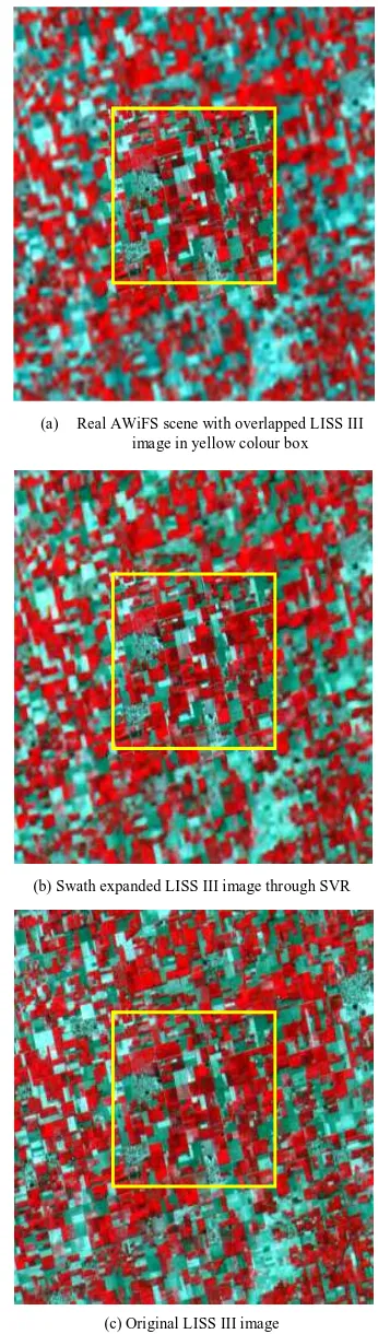
Figure 10(a) is the simulated AWiFS image with overlapped LISS III image in yellow colour box, Figure 10(b) is the swath expanded LISS III using CCL and Figure 10(c) is the original LISS III image. Quantitative results are shown in Table 3. An average RMSE of four bands is 0.0118 in reflectance values. The SAM value is 2.841 in degrees. The SSIM provides the local structural information of an image. An average SSIM of the four bands is 0.91.

Table 3. Quantitative results of single-image-super resolution approach through an SVR.

(c)

Figure 10. Enhancement of AWiFS spatial resolution to the spatial resolution of LISS III in the non-overlapping region by an SVR.

The prediction accuracy is evaluated with the statistical parameter . The prediction accuracy for each band is shown in Figure 9. An average of four bands is 0. 87 i.e. the prediction accuracy of the single-super-resolution approach through SVR

B2 B3 B4 B5

RMSE(reflectance) 0.0097 0.0143 0.0163 0.0070 SSIM 0.90102 0.8956 0.8741 0.8552

(a) Real AWiFS scene with overlapped LISS III image in yellow colour box

(b) Swath expanded LISS III image through SVR

(c) Original LISS III image Quality

parameter

Bands

(a) (b)

(c) (d)

(8)

for the real AWiFS and LISS III data sets is 87% for this experimental data.

5. CONCLUSION

In this paper, we propose two novel approaches to emulate the LISS III images at 740 km swath, 23.5 m spatial and 5-days temporal resolutions. First approach is to emulate the synthetic LISS III images at 23.5 m spatial and 5-days temporal resolutions. Mosaic such images to cover the full 740 km swath of AWiFS for a given date. First approach is achieved through the spatio-temporal data fusion technique which depends on the previously acquired single AWiFS-LISS III image pair. Second approach assumes that the non-overlapping region of AWiFS contains the similar land-cover features of LISS III overlapping region. Then it is possible to enhance the spatial resolution of AWiFS to the spatial resolution of LISS III in the non-overlapping region. It is achieved through a single-image-super resolution technique over contourlet coefficients learning and support vector regression. The effect of second approach is evaluated for simulated and real data sets of AWiFS and LISS III images. But it works well for the data sets which are satisfying the above basic assumption. First approach is computationally efficient but it faces radiometric issues in the mosaic process. Second approach has high computational complexity. An accuracy of both methods is validated with originally acquired LISS III data sets. Experimental results demonstrated that the accuracy of first approach is around 92%, the second approach is around 87% for real datasets, and 92% for the simulated data sets. In second approach, only the overlapping regions of AWiFS and LISS III are used as prior knowledge. The accuracy of this method can be improved by increasing the database of the relevant prior knowledge.

ACKNOWLEDGEMENT

This research was done under technology development project (TDP) at national remote sensing centre, ISRO, department of space, government of India, through a project code: 0606322EE301.

REFERENCES

Chang, C. C., & Lin, C. J., 2011. LIBSVM: a library for support vector machines. ACM Transactions on Intelligent Systems and Technology (TIST), 2(3), pp. 27.

Da Cunha, A. L., Zhou, J., & Do, M. N., 2006. The nonsubsampled contourlet transform: theory, design, and applications. Image Processing, IEEE Transactions on, 15(10), pp. 3089-3101.

Do, M. N., & Vetterli, M., 2005. The contourlet transform: an efficient directional multiresolution image representation. Image Processing, IEEE Transactions on, 14(12), pp. 2091-2106.

Gajjar, P. P., & Joshi, M. V., 2010. New learning based super-resolution: use of DWT and IGMRF prior. Image Processing, IEEE Transactions on, 19(5), pp. 1201-1213.

Gao, F., Masek, J., Schwaller, M., & Hall, F., 2006. On the blending of the Landsat and MODIS surface reflectance: Predicting daily Landsat surface reflectance. Geoscience and Remote Sensing, IEEE Transactions on, 44(8), pp. 2207-2218.

Hall, D. L., & McMullen, S. A. H., 1992. Mathematical techniques in multisensor data fusion. Boston, MA: Artech House.

Hilker, T., Wulder, M. A., Coops, N. C., Seitz, N., White, J. C., Gao, F.,& Stenhouse, G., 2009a. Generation of dense time series synthetic Landsat data through data blending with MODIS using a spatial and temporal adaptive reflectance fusion model. Remote Sensing of Environment, 113(9), pp. 1988-1999.

Hilker, T., Wulder, M. A., Coops, N. C., Linke, J., McDermid, G., Masek, J. G.,& White, J. C., 2009b. A new data fusion model for high spatial-and temporal-resolution mapping of forest disturbance based on Landsat and MODIS. Remote Sensing of Environment, 113(8), pp. 1613-1627.

Huang, B., & Song, H., 2012. Spatiotemporal reflectance fusion via sparse representation. Geoscience and Remote Sensing, IEEE Transactions on, 50(10), pp. 3707-3716. environments with IKONOS imagery: enhanced spatial resolution can deliver greater thematic accuracy. Remote sensing of environment, 82(2), pp. 248-257.

Pohl, C., & Van Genderen, J. L., 1998. Review article multisensor image fusion in remote sensing: concepts, methods and applications. International journal of remote sensing, 19(5), pp. 823-854.

Rao, C. V., J. Malleswara Rao, A. Senthil Kumar, V. K. Dadhwal, 2014a. Fast Spatio-temporal Data Fusion: Merging LISS III with AWiFS Sensors Data, International Journal of Remote Sensing [In press].

Rao, C. V., J. Malleswara Rao, A. Senthil Kumar, B.Lakshmi,V. K. Dadhwal, 2014b. Expansion of LISS III Swath using AWiFS Wider Swath Data and Contourlet Coefficients Learning, GIScience and Remote Sensing Journal [In press].

Rao, C. V., Rao, J. M., Kumar, A. S., & Manjunath, A. S. , 2011. Restoration of high frequency details while constructing the high resolution image. In India Conference (INDICON), 2011 Annual IEEE, pp. 1-5

Rao, C. V., Rao, J. M., Kumar, A. S., Jain, D. S., & Dadhwal, V. K., 2014c. Satellite image fusion using Fast Discrete Curvelet Transforms. In Advance Computing Conference (IACC), 2014 IEEE International, pp. 952-957

Song, H., & Huang, B., 2013. Spatiotemporal satellite image fusion through one-pair image learning. Geoscience and Remote Sensing, IEEE Transactions on, 51(4), pp. 1883-1896.

Wang, Z., Bovik, A. C., Sheikh, H. R., & Simoncelli, E. P., 2004. Image quality assessment: from error visibility to structural similarity. Image Processing, IEEE Transactions on, 13(4), pp. 600-612.