Economics of Education Review 18 (1999) 311–325
Community effects and desired schooling of parents and
children in Mexico
Melissa Binder
*Department of Economics, University of New Mexico, 1915 Roma NE–SSCI 1019, Albuquerque, NM 87131-1101, USA
Received 1 November 1996; accepted 1 July 1998
Abstract
This paper investigates community effects in the determination of desired schooling in a sample of more than 300 school children and their parents in three Mexican cities. Community residence is found to be a significant predictor of desired schooling of parents and children, even with comprehensive controls for child and family traits. Measurement error and omitted variable bias are considered, but rejected, as principal causes of this result. A comparison of recent and long-term residents of a community reveals that the predictive power of residence is much stronger for long-term residents. This result is interpreted as evidence of community effects, since the alternative hypothesis of Tiebout behavior predicts a stronger common effect for recent migrants. Potential sources of the community effects are then investigated with neighborhood-level data from the 1990 Mexican Census. 1999 Elsevier Science Ltd. All rights reserved.
Keywords:Community effects; Education in developing countries
We wanted our children to continue studying, but they saw their friends in the streets, and working, and they didn’t want to go to school any more (Mother in El Cerro del Cuatro, Guadalajara).
1. Introduction
It is widely acknowledged that family characteristics such as household income and parent schooling affect the costs and benefits of schooling. A wealthy family can finance the costs of schooling internally—and therefore more cheaply—than a family borrowing externally. A better educated parent may have more knowledge about the schooling system, lowering the cost of collecting information about it. Similar reasoning also holds for community characteristics. For example, consider a
com-* Tel.: 11-505-277-5304; fax: 11-505-277-9445; e-mail: [email protected]
0272-7757/99/$ - see front matter1999 Elsevier Science Ltd. All rights reserved. PII: S 0 2 7 2 - 7 7 5 7 ( 9 8 ) 0 0 0 3 7 - 5
munity that has no neighborhood high school, and few residents who ever attended high school. In this com-munity the costs of learning how to enroll in high school will be relatively high.
Described in this way, the neighborhood characteristic itself helps to explain behavior. But the contention that neighborhoods “matter”—or that true community effects exist—is controversial. The problem is that people are not randomly assigned to their neighborhoods: they choose them for a reason. Presumably if parents plan to send their children to high school, they will look for a neighborhood that has one nearby. Children living in neighborhoods without high schools may have difficulty in attending them, not because their parents face large costs in getting information about them, but because their parents didn’t value education enough in the first place to move into a neighborhood that had one. This is the gist of the argument of Tiebout (1956), that like people self-select into the same neighborhoods.
schooling outcomes if community effects exist. But if Tiebout behavior dominates, where a child goes to school should make little difference.
Unfortunately, the two theories are difficult to dis-tinguish empirically, since a finding that communities matter does not rule out the possibility of an unobserved trait that all families in the community share (Jencks & Mayer, 1990; Manski, 1993). In this case, The shared trait matters, and not the communityper se1.
Neverthe-less, as Jencks and Mayer (1990) argue, the community effects and Tiebout theories predict opposite effects for length of residence. If the community matters, then pre-sumably it will matter more over time: new-comers will be less affected by it. If self-selection matters, then the community trait will describe new-comers best, since they are choosing where to live now, as the community exists today, and long-term residents may have made their choice under different community conditions. In applying this distinction to a new data set that records the desired schooling of Mexican school children and their parents, I find evidence for true community effects: the desired schooling of recent migrant adults for their children is not significantly predicted by their communi-ties, whereas for long-term resident adults, community residence is a highly significant predictor.
I begin by setting out the theoretical importance of desired schooling and the potential role of community effects in its determination. I then present the data and explore the empirical content of desired schooling. I find that desired schooling is largely determined by com-munity fixed effects. These effects cannot be explained by measurement error or omitted variable bias, and, through the length of residence test, appear to reflect true community effects. Finally, I investigate the cause of these effects by using neighborhood-level data from the Mexican Census. Schooling and income levels of the community are significant predictors of desired school-ing, but school enrollment figures for neighborhood youth are not.
2. Demand for schooling, desired schooling, liquidity constraints and neighborhoods
I follow standard human capital theory in treating schooling as a personal investment in a future income
1Summers and Wolfe (1977), Dachter (1982), Case and Katz
(1991), Crane (1991) and Borjas (1992, 1995) claim to find true community effects. Evans, Oates and Schwab (1992) endo-genize the location decision and find no community effects.
stream (Schultz, 1963; Becker, 1964; Mincer, 1974)2.
The optimal desired schooling decision, S*
i, meets the
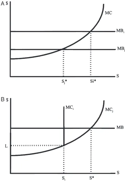
where the left-hand side is the discounted marginal bene-fit and C is the marginal cost of an additional year of schooling. The termdis typically the wage differential earned for the next unit of schooling, but may also include the marginal consumption value. The termd is the rate of time preference, and N is planned working years. These parameters are subscripted to indicate that they may vary for each investori. A simple formulation, where the wage differential reflects a constant return on human capital and a correspondingly constant marginal benefit schedule, is illustrated in Fig. 1(a)3. Marginal
costs rise with years of schooling because both direct costs (especially tuition) and opportunity costs (foregone wages) increase for more advanced students. Fig. 1(a) also shows that the optimal schooling level will vary among students depending on the positions of the mar-ginal benefit and marmar-ginal cost curves. These in turn depend on individual values ofd,d,NandC: low values ofdand high values ofdandNresult in a higher mar-ginal benefit and more schooling; low C values (not shown) would lower the marginal cost curve and also lead to more schooling.
The ability of students to invest in optimal schooling levels depends on their ability to finance direct and indirect costs. Liquidity constraints arise because mar-kets are not available to provide unsecured loans on human capital investments. For this reason, a student’s family background, especially the family’s willingness and ability to finance schooling, will alter schooling out-comes (Becker, 1964). In Fig. 1(b), familyican provide at mostLdollars for schooling, and so faces a vertical marginal cost curve at L. Schooling attainment for a
2Generally, studies of schooling determinants in developing
countries use a household production framework that includes leisure and consumption for all family members, and schooling for children. Schooling is included because parents care about the “quality” of their children, which is measured by children’s future earnings. But, while parents care about future income, they are not making an investment decision: schooling is treated like an ordinary consumption good. See, for example, Rosenzweig and Evenson (1977), King and Lillard (1983), Birdsall and Cochrane (1982), Wolfe and Behrman (1984), Birdsall (1985) and Handa (1996). Behrman and Wolfe (1987) and Glewwe and Jacoby (1994) are two studies that appeal to the investment model.
3The conclusions from this analysis do not depend on the
Fig. 1. Optimal schooling investments and liquidity con-straints. a: No liquidity constraints; different investors face dif-ferent marginal benefits schedules depending on individual schooling differentials, time preferences and working horizons. b: Investment with binding liquidity constraints reduces attained schooling. Familyiexhausts its resources and is constrained to stop school atSi. In familyj the liquidity constraint does not
bind and schooling continues untilS*.
child in this family falls short of optimal desired school-ing.
The presence of liquidity constraints is likely to coincide with a higher marginal cost curve, so that desired schooling will be related to realized school attainment. In poor families, parents face both direct and opportunity costs of schooling. In wealthy families, a child’s opportunity wages are likely to be a tiny fraction of the family budget so that, in some sense, the family does not face them. Thus even when liquidity constraints bind, we would expect that desired schooling would be correlated with schooling eventually attained.
The foregoing discussion points to the relevance of desired schooling both as an integral part of schooling demand and also in terms of contributing to schooling outcomes, even in the presence of liquidity constraints. What role, if any, might the community have in determining desired schooling? Community conveys the meaning of something common to all members, some-thing shared. The most basic some-thing that can be shared is
a geographic area: families living next to each other share the same external environment, including the same local establishments and institutions, such as schools and churches. Social relations are likely to arise from this sharing, be they friendships or conflicts. Anthropological studies suggest that extra-family friendships and net-works of reciprocal exchange abound in Mexican neigh-borhoods (Lewis, 1959; Lomnitz, 1977). While com-munities under this definition may span neighborhoods, I assume here that sources of community effects, both social and institutional, arise within neighborhoods.
The community effects literature suggests four poss-ible mechanisms by which neighborhoods might have independent effects on individual outcomes such as desired schooling, apart from and in addition to family and personal effects. First, there may be different market and institutional resources in different neighborhoods. For example, a rural community might have more opportunities for child labor; an urban community might have better schools. The former would raise the marginal cost of schooling; the latter would lower it. Second, com-munities might form the basis for information about labor market opportunities and schools. There may be less of this information available in neighborhoods where few have studied beyond primary school (Wilson, 1987). This mechanism would raise marginal schooling costs by increasing the costs of collecting information. Third, communities may provide social networks that are useful in locating jobs (Montgomery, 1991). Marginal benefits might be higher in neighborhoods with good connections. Finally, peer effects, also discussed in the literature as epidemic theory (Crane, 1991) and tipping models (Schelling, 1978), suggest that people behave as the majority of their peers do, regardless of family back-ground. With peer effects, there may be social costs to pursuing goals that are not the norm, or added benefits from pursuing goals that are. The remarks of the mother quoted at the beginning of this article are emblematic of a neighborhood peer effect.
3. A survey of Mexican school children and their families
manufacturing center of domestically distributed con-sumer non-durables with a population of three million. Arandas is a small city of 30 000 that is a commercial center for the agricultural activity that surrounds it. Tijuana is a center of export-oriented maquiladora plants with 750 000 residents4. Students in these different cities
face distinct labor markets, although the possibility of migration (especially from Arandas to Guadalajara) may blur the distinction5.
The fifth grade was chosen as a compromise between two methodological concerns. First, since the purpose of the survey was to explore determinants of schooling among those with the lowest educational attainment, and drop-out rates are high even in primary school, students needed to be relatively young. (The primary school efficiency rate—the ratio of graduates to entrants six years earlier—was only 55% in the 1990–91 school year, as reported by the Secretarı´a de Educacio´n Pu´blica, 1986, 1991.) Second, students also needed to be mature enough to have some idea of their future plans and the ability to report accurately on basic information about their households. The sample, then, is restricted to chil-dren who have not dropped out of school as of the fifth grade and therefore contains potential sample selection bias against those with less schooling. The 1990 Census reports that 13% of children 15–19 years of age had attained four years of schooling or less. This figure com-bines urban and rural residents, and probably overesti-mates low attainment among urban children.
The sample schools were selected by their location in neighborhoods of varying income levels. Since all chil-dren in a randomly selected fifth grade class were inter-viewed6, and children typically attend the school closest
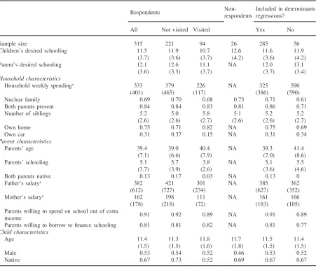
to them, the sample represents neighborhood families with school-age children. Most parents answered a ques-tionnaire sent home with their children; we directly inter-viewed 94 non-responding parents in their homes. Table 1 compares the characteristics of households who responded independently with those who were visited. Parents in the visited sample were poorer and less edu-cated than those who answered independently. They were also more likely to be migrants. Both parents’ and children’s desired schooling in visited households were more than a year lower than desired schooling in inde-pendently responding households.
We were unable to collect information for the parents
4Populations are drawn from the Jalisco and Baja California
state volumes of the 1990 Mexican Census of Population and Housing.
5Most of the Arandas children had relatives in Guadalajara,
which is only a two-hour bus ride away.
6I was the sole interviewer for the schools in Guadalajara
and Arandas, and was ably assisted by Universidad Auto´noma de Baja California student Hector Gutı´errez in Tijuana.
of 26 of the interviewed children. The bulk of these (11) are parents from the private school, where non-respon-dents were not visited at their homes at the request of the school’s director. Although the private school sample is probably less prone to selectivity bias with respect to selection against less educated parents, the sample may have systematically excluded wealthier parents. Table 1 shows that children of non-responding parents desire more schooling on average than the rest of the sample. An additional 30 observations are omitted from the analyses of determinants of schooling desires because they are missing one or more variable values. Table 1 shows that this group tends to have higher desired schooling of parents and children, and more income. If many children with high incomes and high schooling desires are excluded, the estimated effect of income may be biased downward. Other characteristics of the excluded group are not very different from those included in the regressions.
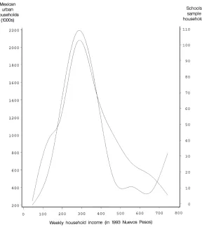
The data share broad characteristics with the general urban Mexican population7. Fig. 2 compares frequency
distributions for a 1988 national sample of urban house-holds (Inegi, 1992b) with the schools sample by weekly income levels. Income for the national sample is reported as multiples of the minimum salary; the 1993 minimum salary was used in the conversion from minimum salaries to pesos8. The distribution from my survey approximates
the national distribution, especially for families of mod-est means. It does, however, undersample the upper end of the distribution. National education levels for urban adults also suggest that my sample is not unusual: about half of men and women in the same age groups as the surveyed parents had completed six years or less years of schooling in 1992 (Inegi, 1993).
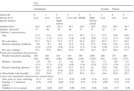
Table 2 presents the data by sample schools, which are characterized (in the first row) by income level. The Guadalajara schools show patterns of rising years of desired schooling with rising income levels. The low-income community sample in the small town of Arandas is indistinguishable in its socio-economic characteristics from the low-income samples in Guadalajara, except for a larger proportion of merchants in the occupational dis-tribution (not shown).
The Tijuana school samples fall between the low- and low–middle- income samples in Guadalajara in child labor-force participation, household spending, and mother’s education in Table 2. In terms of occupational distribution, Tijuana is also very similar to the low-income Guadalajara samples. Ax2test cannot reject the
null hypothesis that the occupational distributions for the
7According to the 1990 national census, 71% of the Mexican
population is urban.
8The minimum salary in 1993 was N$92, or about US$30,
Table 1
Summary statistics for respondents and non-respondents (standard deviation in parentheses)
Non- Included in determinants Respondents
respondents regressions?
All Not visited Visited Yes No
Sample size 315 221 94 26 285 56
Children’s desired schooling 11.5 11.9 10.7 12.6 11.6 11.9
(3.7) (3.6) (3.7) (4.2) (3.6) (4.2)
Parent’s desired schooling 12.1 12.6 11.1 NA 12.0 13.1
(3.6) (3.5) (3.7) (3.7) (3.4)
Household characteristics
Household weekly spendinga 333 379 226 NA 325 590
(401) (465) (117) (386) (590)
Nuclear family 0.69 0.70 0.68 0.73 0.71 0.61
Both parents present 0.84 0.84 0.83 0.81 0.86 0.71
Number of siblings 5.2 5.0 5.8 5.1 5.2 5.2
(2.6) (2.6) (2.7) (2.6) (2.6) (2.7)
Own home 0.75 0.71 0.82 NA 0.75 0.69
Own car 0.31 0.37 0.15 NA 0.31 0.34
Parent characteristics
Parents’ age 39.4 39.0 40.4 NA 39.3 41.4
(7.1) (6.6) (7.9) (7.0) (8.6)
Parents’ schooling 5.1 5.7 3.8 NA 5.1 5.5
(3.7) (3.9) (2.6) (3.6) (4.6)
Both parents native 0.13 0.17 0.03 NA 0.13 0
Father’s salarya 382 421 301 NA 385 362
(612) (727) (234) (627) (352)
Mother’s salarya 162 198 111 NA 161 166
(178) (218) (72) (183) (105)
Parents willing to spend on school out of extra
0.91 0.92 0.89 NA 0.91 0.89
income
Parents willing to borrow to finance schooling 0.81 0.81 0.82 NA 0.81 0.77 Child characteristics
Age 11.4 11.3 11.8 11.7 11.5 11.4
(1.5) (1.5) (1.6) (1.8) (1.5) (1.5)
Male 0.53 0.54 0.52 0.46 0.53 0.52
Native 0.67 0.73 0.52 0.69 0.67 0.67
All statistics between 0 and 1 indicate sample proportions for this characteristic.
aIn nuevos pesos, which exchanged at about three per US$ at the time of the survey (in 1993).
low-income Guadalajara, Arandas and Tijuana samples are the same. But in years of desired schooling, the Tiju-ana children break ranks with the low- and low–middle-income Guadalajara children. As indicated in Table 2, the Tijuana children are very aspiring; desired schooling levels match or exceed those of middle-income Guadala-jara children. A x2test rejects the null hypothesis that
the Tijuana samples have the same desired schooling dis-tribution as the other low-income samples.
4. Can we measure desired schooling?
According to the investment framework, students may attain less than their desired schooling due to liquidity
over-Fig. 2. Frequency distribution of Mexican urban households by income level: national and schools samples. Sources: Inegi (1992b) and author’s schools survey.
report schooling desires in an effort to provide what might have been perceived as the socially desirable answer. In addition, survey designers are familiar with the tendency of survey participants to represent them-selves in a positive light, whatever the institutional back-ing of the survey9.
Students and parents responded to a series of questions about their desired schooling levels. They were first asked outright the school level and grade they wanted to achieve. They were later asked what they wanted to do upon finishing their studies. The vast majority (all but four) who planned to work in the labor force were asked their occupational preference, and what they thought the required schooling to get a job in this occupation would be. To mitigate against the tendency to over-report, desired schooling used in the analyses to follow is the lower of the outright and occupation responses. The idea is that the more specific occupational response introduces
9Sudman and Bradburn (1982), for example, cite
consider-able over-reporting of having a public library card, in a study where responses were verified in library records.
a “reality check” on children’s and parents’ true desired schooling. Twenty-two per cent of the children and 17% of the parents were ascribed their occupation responses. These children and parents also reported lower house-hold spending and parent schooling levels. The mean of the constructed desired schooling measure was lower and the standard deviation higher than the outright desired schooling response10.
Participants were also asked if they thought their desired schooling levels were likely to be realized and what potential obstacles they expected to encounter. Close to one-half of the children and about two-thirds of parents expected financial difficulties in achieving desired schooling levels.
The data in Table 1 show that there is considerable variation in reports of desired schooling. For the sample as a whole, mean desired schooling of children is 11.5
10The means (and standard deviations) for children’s
Table 2
Summary statistics by school (standard deviations in parentheses) City
Guadalajara Arandas Tijuana
School ID 0 1 2 3 4 6 7 8 9
Income level Low Low Low Low–mid Middle High Low Low Low
Special features Night Private
school school
Students/classa 43.2 49.3 45.3 39.1 35.0 24.8 37.6 40.5 34.3
Students surveyedb 37 40 38 36 37 31 43 41 38
Children’s characteristics
Age 11.5 11.6 13.9 11.1 10.7 11.1 11.5 10.8 10.8
(1.1) (1.3) (2.1) (1.0) (1.0) (0.8) (1.2) (1.1) (1.0)
Per cent native 91.7 74.4 73.7 72.2 91.9 45.2 83.7 31.7 34.2
Desired schooling (children) 9.8 9.7 8.6 11.4 13.6 15.3 10.0 13.8 13.0
(3.4) (3.3) (3.0) (3.4) (2.7) (1.8) (3.0) (3.1) (3.2)
Per cent workingc 35.1 35.0 69.4 25.0 19.4 12.9 44.2 26.8 23.7
Parent and household characteristics
Weekly household spending 204 188 219 339 350 1488 204 275 286
(62) (86) (106) (289) (219) (1187) (93) (110) (137)
Mothers’ schooling 3.9 2.9 2.7 5.6 8.0 12.2 3.2 6.0 5.2
(3.1) (1.7) (2.3) (4.0) (3.8) (2.9) (2.7) (2.9) (3.3)
Desired schooling (parents) 10.3 10.2 10.7 12.2 14.5 16 10.8 14.0 12.7
(3.3) (3.3) (3.6) (3.6) (2.7) (0) (3.7) (2.7) (3.2)
% Households with benefitsd 18.9 25.0 27.7 24.2 39.4 42.1 14.6 45.0 39.5
Census-tract population characteristics (proportions)
Nine years or more schooling 0.11 0.11 0.17 0.54 0.49 0.74 0.23 0.32 0.32
Earning#2 minimum 0.70 0.70 0.69 0.45 0.55 0.35 0.69 0.53 0.53
salaries
Children 6–14 in school 0.85 0.85 0.87 0.90 0.93 0.96 0.86 0.77 0.78
aThis is an average for all classes in the school.
bIn the private school, children are a sample from two classes. In all other schools, all children in one fifth-grade class were
inter-viewed.
cOr actively seeking work.
dBenefits received through employment of either or both parents.
years, with a standard deviation of 3.7 years. For parents, the mean and standard deviation are 12.1 years and 3.6 years, respectively. In Table 2, reports of desired school-ing vary considerably among the sampled schools, with means of 15 and 16 years for children and parents, respectively, in the private school, compared with 10 and 11 years in Arandas. This is particularly reassuring given that parents chose a response from a list of possible attainments that culminated at the university level11.
From the framework set out in Section 2, schooling attainment should be positively associated with desired schooling and negatively associated with measures of liquidity constraints. Analysis of the available data sug-gests that this is the case. Since the sample children are
11Reported desired schooling levels were translated into
years as follows: primary school56 years; middle school5
9 years; high school512 years; university516 years.
still in school, their eventual schooling attainment is not known. However, the survey also reported the age, sex and schooling attainment for siblings, many of whom have completed their schooling12. A Tobit analysis can
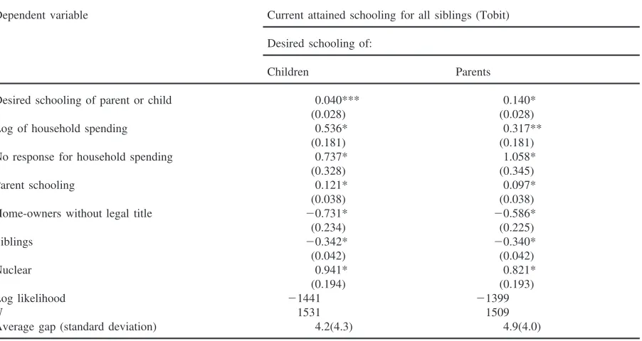
use information from both the completed schooling of older siblings and the right-censored schooling of sample children and siblings still in school to assess the determi-nants of eventual schooling attainment. Table 3 presents the results of a Tobit that models schooling attainment as a function of desired schooling, income and wealth measures and family background traits. Estimates of the effect of desired schooling are likely to be noisy, since the model implicitly ascribes the desired schooling of parents for the sample child to all their other children,
12Ninety-six per cent of the surveyed children have siblings
Table 3
Models of expected schooling using current attainment of all siblings in a Tobit modela(standard errors in parentheses)
Dependent variable Current attained schooling for all siblings (Tobit) Desired schooling of:
Children Parents
Desired schooling of parent or child 0.040*** 0.140*
(0.028) (0.028)
Log of household spending 0.536* 0.317**
(0.181) (0.181)
No response for household spending 0.737* 1.058*
(0.328) (0.345)
Parent schooling 0.121* 0.097*
(0.038) (0.038)
Home-owners without legal title 20.731* 20.586*
(0.234) (0.225)
Siblings 20.342* 20.340*
(0.042) (0.042)
Nuclear 0.941* 0.821*
(0.194) (0.193)
Log likelihood 21441 21399
N 1531 1509
Average gap (standard deviation) 4.2(4.3) 4.9(4.0)
aModels also include dummy variables for renters and those living in rent-free arrangements with relatives or others, so that
coefficients for home-owners without legal title are relative to home-owners with legal title. Models also control for age, age-squared and gender.
*Significant at the 5% level. **Significant at the 10% level. ***Significant at the 20% level.
and, worse, the sample child’s desired schooling for him-or her self to his him-or her siblings. Nevertheless, parents’ desired schooling is a significant and positive predictor of schooling attainment13; children’s desired schooling is
a positive but weak predictor. Likely measures of bind-ing liquidity constraints are negatively associated with schooling attainment. Spending (a proxy for permanent income) enters the model positively and significantly (at the 5% and 10% confidence levels for children and par-ents, respectively). Dummy variables for homeowners without legal title–who would presumably be unable to use their property as collateral for loans—have a
statisti-13The relationship between aspirations and attainment has
been studied widely in the sociological literature. In US data, schooling “aspirations” are found to be statistically significant predictors of eventual educational attainment (Portes & Wilson, 1976; Thomas, 1980; Sewell, Hauser & Wolf, 1980). Jamison and Lockheed (1987), in a rare study that considers the effect of desired schooling and attitudes on schooling in a developing country, find that parents’ desired schooling has a significant effect on their children’s school enrollment in Nepal.
cally negative effect at standard confidence levels14. In
sum, the model performs as expected, with desired schooling of parents playing a significant positive role in determining eventual schooling attainment.
5. School sample fixed effects and community effects
I now estimate the extent to which the variation in desired schooling is systematically related to personal, family and community characteristics of children and parents with the following linear model:
Si,j,k5b01b1Ij1b2Fj1b3Ck1ck1ui,j (2)
where desired schoolingSi,j,k of student (or parent)iin
familyjand communitykis a linear combination of vec-torsI and Fwhich contain child and family
character-14A model that controls for many more family traits, as well
istics, respectively, and a vector of dummy variablesC that take the value of 1 if the observation is drawn from a given school sample, and 0 otherwise; b1,b2 and b3
are vectors of coefficients andb0is a constant term; ck
is a common error term for all observations in a given school sample, andui,j is an error term for personi in
familyj15 16.
Child characteristics include age, sex, whether the child was born in the survey city (native) or not, and birth order. Family background variables include parent schooling and age, a measure of income, number of sib-lings, family structure (nuclear or extended) and dummy indicators for the occupation of the household head. Weekly household spending rather than earnings is used as the income measure because it should be a better proxy for permanent income17. Permanent income, in
turn, is a better measure of a household’s economic status than current income, and is especially relevant for investment behavior18. In addition, several variables that
measure parent attitudes toward schooling are included. Parents were asked if their children would receive more schooling (1) if they enjoyed higher incomes and (2) if they could borrow to finance schooling. Finally, parents’ desired schooling is also used as an independent variable in models of children’s desired schooling.
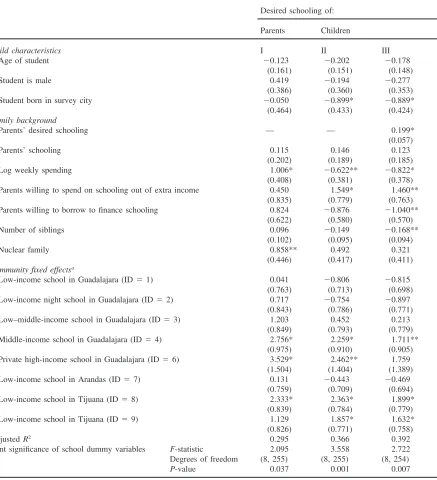
Table 4 shows that the community dummies are sig-nificant predictors of desired schooling for both parents and children, even in the presence of detailed family characteristics. Relative to the omitted low-income Gua-dalajara school sample, being in a middle-income, high-income or Tijuana school has a large, positive and sig-nificant effect on years of desired schooling for both par-ents and children, even after controlling for income and
15The investment model implicitly relies on investors’
per-ceived and likely uncertain benefits of schooling. The survey did not produce adequate measures of the access to accurate information about future earnings. The survey did include a question about how difficult parents and children felt it would be to find employment in the desired fields. Presumably, dif-ficulty in finding employment would lead to lower expected benefits. The measure of the probability of employment, though, had no statistical significance when it was included in specifi-cations not reported here.
16This specification does not allow the model parameters to
vary among schools. Although results reported in what follows suggest that the parameters do in fact vary, a comprehensive multi-level analysis is not possible, given the limited number of schools in the sample.
17The most common occupation reported for household
heads was construction worker. Construction jobs are usually temporary and often seasonal. The wage reported in any given week is unlikely to be an accurate measure of permanent income.
18The variables included are standard in the determinants of
schooling literature; see footnote 2 for research that follows this approach.
other individual and family characteristics. Desired schooling for children in the middle-income Guadalajara school is 1.7 years higher than for children in low-income schools in Guadalajara and Arandas. Desired schooling for Tijuana children is between 1.6 and 1.9 years higher. Coefficients on school dummy variables are even larger for parents, where parents in the high-income communities desire three more years of schooling for their children than do parents in low-income communi-ties.
What is causing these large estimates for school sam-ple fixed effects? As summarized earlier, one interpret-ation is that the fixed effects are community effects that exert an independent effect on the behavior of com-munity members. The alternative hypothesis is that the large estimated fixed effects are simply proxies for unob-served, but shared, family characteristics. The fixed effect will then be caused by Tiebout behavior in which “like” people group themselves in communities.
I first consider some spurious possible causes of the fixed effects and then examine how well the data fit the implications of each hypothesis. I begin by establishing the overall significance of the school dummy variables. F-tests reject the hypothesis of zero joint significance of the dummy variables for both children and parents (see Table 4).F-tests also reject pooling of all samples: poo-ling is accepted for the low-income school samples in Guadalajara and Arandas, and for the remaining schools which include the higher-income Guadalajara groups and the Tijuana schools19. This division roughly follows the
distinction between schools that have significantly differ-ent coefficidiffer-ents on the school sample dummies and those that do not.
The school dummies do seem to be providing infor-mation. It is possible, though, that the school dummies are providing information about imprecisely measured or unobserved family characteristics. Measurement error is unlikely, due to the high degree of control I had in col-lecting data. I nevertheless consider its presence by cal-culating what bias it would introduce in the estimated coefficients, following the approach of Borjas (1992). Assume that the true model depends only on a family background measure and no community measures. In this case, if the available family and community vari-ables are imperfect proxies for the true family measure, then we estimate:
Sj,k5b01u1Fj*1u2Ck1uj,k (3)
whereF* is a family characteristic measured with error
19In order to increase the degrees of freedom and so have
Table 4
Point estimates of determinants of desired schooling for parents and children (standard errors in parentheses) Desired schooling of: Parents Children
Child characteristics I II III
Age of student 20.123 20.202 20.178
(0.161) (0.151) (0.148)
Student is male 0.419 20.194 20.277
(0.386) (0.360) (0.353)
Student born in survey city 20.050 20.899* 20.889*
(0.464) (0.433) (0.424)
Family background
Parents’ desired schooling — — 0.199*
(0.057)
Parents’ schooling 0.115 0.146 0.123
(0.202) (0.189) (0.185)
Log weekly spending 1.006* 20.622** 20.822*
(0.408) (0.381) (0.378)
Parents willing to spend on schooling out of extra income 0.450 1.549* 1.460**
(0.835) (0.779) (0.763)
Parents willing to borrow to finance schooling 0.824 20.876 21.040**
(0.622) (0.580) (0.570)
Number of siblings 0.096 20.149 20.168**
(0.102) (0.095) (0.094)
Nuclear family 0.858** 0.492 0.321
(0.446) (0.417) (0.411)
Community fixed effectsa
Low-income school in Guadalajara (ID51) 0.041 20.806 20.815
(0.763) (0.713) (0.698)
Low-income night school in Guadalajara (ID52) 0.717 20.754 20.897
(0.843) (0.786) (0.771)
Low–middle-income school in Guadalajara (ID53) 1.203 0.452 0.213
(0.849) (0.793) (0.779)
Middle-income school in Guadalajara (ID54) 2.756* 2.259* 1.711**
(0.975) (0.910) (0.905)
Private high-income school in Guadalajara (ID56) 3.529* 2.462** 1.759
(1.504) (1.404) (1.389)
Low-income school in Arandas (ID57) 0.131 20.443 20.469
(0.759) (0.709) (0.694)
Low-income school in Tijuana (ID58) 2.333* 2.363* 1.899*
(0.839) (0.784) (0.779)
Low-income school in Tijuana (ID59) 1.129 1.857* 1.632*
(0.826) (0.771) (0.758)
AdjustedR2 0.295 0.366 0.392
Joint significance of school dummy variables F-statistic 2.095 3.558 2.722 Degrees of freedom (8, 255) (8, 255) (8, 254)
P-value 0.037 0.001 0.007
Models were estimated with PROC REG in SAS for 286 observations, and included a constant term and a dummy variable for each school, as well as the following controls: the square of parents’ schooling, average of parents’ years of age, relative birth order (early, middle or late, relative to only-children), a dummy variable for observations where no spending value was reported (if so, average spending for the school sample was used), and dummy variables for seven occupational groups.
aOmitted school is a low-income school in Guadalajara (ID50).
and C is a community characteristic, when the real model is
Sj5b01b1Fj1uj (4)
The trueFis equal toF*1v2, andCimperfectly
meas-uresFso thatCis equal toF1v3.v2andv3are random
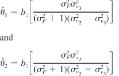
error terms. An OLS estimate of Eq. (3) will give us the following biased estimates.
v3 are the variations of the error terms
v2andv3, respectively. It follows that
ifs2
v3>s
2
v2thenuˆ1>uˆ2
If the measurement error of the community proxy for the true family trait is larger than the measurement error of the family proxy for this trait—as might be expected— then the coefficient of the family characteristic will be larger than the coefficient of the community character-istic. In fact, estimated coefficients for school sample means and census measures of household income and parent schooling are larger than the coefficients for the corresponding family measures. (Table 6 provides this comparison for random effects estimates. The results were the same using OLS.) In order to accept that the results are driven by measurement error, one would have to accept that mean community schooling (or spending) is a better measure of parent schooling (or spending) than is the parent’s own report.
I now turn to the possibility of omitted variable bias. Columns 2 and 3 in Table 4 allow a comparison of school sample dummies for children in models that alter-natively omit and include parents’ desired schooling—a variable that is usually “unobserved”. If parents’ desired schooling is a good measure of parent attitudes about schooling, then it is exactly the kind of variable that might be expected to drive the community effects results in a Tiebout world. The inclusion of this variable reduces the size and significance of the sample dummy variables, but F-tests definitively reject the hypothesis that the dummy coefficients are zero in both specifications. The P-value for the model that includes parent desired schooling is 0.007. Thus neither measurement error bias nor omitted variable bias provides convincing expla-nations for the large fixed effects.
Fortunately, the Tiebout and community effects mod-els imply opposite relative strengths of the observed effects for groups according to their length of residence in a particular neighborhood (Jencks & Mayer, 1990). In
the Tiebout model, people “bring” their “fixed effects” with them to a community. If this is true, then we would expect recent migrants to the community to be carrying the shared unobserved trait. Longer-term residents are less likely to have the trait, since the community may have changed considerably since they moved in, and moving out may be costly. The community effects model predicts just the opposite: longer-term residents should be more subject to the “community effects”, for having lived with them that much longer. It is plausible that all of the possible mechanisms for community effects out-lined in Section 2 above (institutional, informational, net-works and peer effects) will be stronger over time.
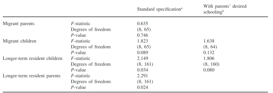
The test of these hypotheses is straightforward. Fixed effects models are estimated separately for recent migrants and longer-term residents, and the significance of the sample dummy variables is then compared. If the community effects hypothesis holds, then we would expect the sample dummy variables to be more predic-tive of desired schooling for the longer-term residents than for migrants. If the Tiebout hypothesis holds, we would expect the opposite result. Unfortunately, data limitations will tend to blur the distinction between recent migrants and longer-term residents. Since length of residence in the current community was not reported, migrant families are identified as such if the child was born outside of the sample city and longer-term residents are identified as such if the child was born in the sample city. Thus those classified as longer-term residents may also include new-comers to the neighborhood. The bias introduced by this measurement problem will tend to make the longer-term residents and recent migrants more similar and so understate the result of a difference between them. This will be especially true for children, since some children born outside of the sample city may have migrated shortly after birth.
Table 5
Joint significance of dummy variables for school samples for recent migrants and longer-term residents
With parents’ desired Standard specificationa
schoolingb
Migrant parents F-statistic 0.635
Degrees of freedom (8, 65)
P-value 0.746
Migrant children F-statistic 1.823 1.638
Degrees of freedom (8, 65) (8, 64)
P-value 0.089 0.132
Longer-term resident children F-statistic 2.149 1.806
Degrees of freedom (8, 161) (8, 160)
P-value 0.034 0.080
Longer-term resident parents F-statistic 2.291 Degrees of freedom (8, 161)
P-value 0.024
aSee columns 1 and 2 in Table 4. bSee column 3 in Table 4.
rises with potential length of residence in the com-munity.
But could this result be caused by the relatively large contribution of migrants from communities that are simi-lar to each other? Consider the coefficient estimates on the community dummy variables in Table 4. School IDs 1, 2, 3 and 7 are not significantly different from the omit-ted school. If migrants come disproportionately from these schools, then the results in Table 5 may be a coincidence. In fact, though, all schools have migrants. Moreover, three of the four schools which exhibit the strongest community effects also have the largest migrant contributions. If there were no real difference in the community effect between migrant and longer-term resident groups, then we would expect that the com-munity dummy variables would be more significant for the migrant sample, which draws more heavily from the distinct communities. Moreover, similar results hold even when the two most migrant communities are omit-ted: longer-term adult residents display significant com-munity effects at the 10% level and no other groups show significant effects20.
Another implication of the community effects
hypoth-20It is also possible that the distinction between recent
migrants and long-term residents (many of whom were early migrants) results from heterogeneity in the more recent migrant pool. Under this possibility, earlier migrants exhibit Tiebout behavior, and more recent migrants—perhaps facing different constraints—do not. Besides an (unknown) exogenous change in the ability to express Tiebout behavior, recent and early migrants migrated in similar proportions from rural and urban source communities from the same areas, and many other rel-evant characteristics—such as schooling and family size—are controlled.
esis is that community level variables—and not just com-munity dummies—should have explanatory power. Data constraints often dictate the size and shape of the com-munity from which characteristics are measured. For example, Behrman and Wolfe (1987) use the percentage of school age children enrolled in school in a munici-pality as a measure of school availability and Birdsall (1985) uses average teacher schooling and salary as a measure of school quality in each of 169 urban and rural areas in Brazil. Dachter (1982) and Corcoran, Gordon, Laren and Solon (1992) use zip code zones. These meas-ures are, at best, ad hoc.
An alternative approach uses group means as inde-pendent community variables. Here researchers may have more leeway in constructing groups. Case and Katz (1991), for example, use means for observations in a two-block radius. The main drawback of using sample means is that they may not accurately represent the over-all community and, in smover-all samples, may be too sensi-tive to individual observations21.
The census tract data I use for community character-istics correspond to the idea of neighborhoods introduced in Section 2 above. Census tracts used by the 1990 Mex-ican Census (Inegi, 1992a) have populations of about 5000 and correspond to geographically integrated and sensibly divided (from my personal observations) neigh-borhoods22.
21In Case and Katz (1991), for example, the measures are
based on at most 15 observations for each two-square block area; in Borjas (1992), some of the ethnic groups used have fewer than 15 observations.
22For two school samples in Guadalajara (the low–middle
The data provide population tabulations from which I can calculate percentages of workers in each neighbor-hood earning different multiples of the minimum salary, school enrollment rates for children of ages six to 14, and proportions of adults who completed different schooling levels for each school sample neighborhood. I also use a direct measure of school quality: the number of stu-dents per class in each school.
In OLS models for children’s desired schooling, three of these community measures increase the variation explained by family and personal characteristics alone by 6% (fromR250.36 toR250.38). In comparison,
the school sample dummies increase explained variation by 9% (to R2 50.39). Thus most of the fixed effects
can be explained by the school quality measure, the pro-portion of neighborhood resident workers earning two minimum salaries or less, and the proportion of adults with nine years of schooling or more in each neighbor-hood. In contrast, these community measures increase variation explained for parents’ desired schooling by less than 1%, compared with an 8% increase when school sample dummies are included.
Table 6 shows how community variables perform when entered separately in a model that includes all the available family and personal characteristics used in the fixed effects models in Table 4. (They are highly corre-lated and so lose significance when entered together.) In addition to the census and school quality measures, I also use school sample means.
Of particular interest is the high predictive value of average community schooling and community earnings. The former indicator may reflect informational, peer or institutional community effects, the latter is likely asso-ciated with institutional effects. For example, communi-ties with relatively low proportions of workers earning two minimum salaries or less are associated with higher levels of desired schooling. The potential importance of this measure may explain why the Tijuana sample has relatively high desired schooling. Although the average weekly spending in Tijuana is only slightly higher than spending in low-income communities elsewhere in the sample, there are also relatively fewer very poor families in Tijuana. If this fact reflects the relatively greater job opportunities in Tijuana, children and parents may per-ceive higher marginal benefits from schooling through greater probability of finding work. Another possibility is that if there is greater demand for skilled workers in Tijuana, returns to schooling may be higher23.
tract characteristics. In some sense, then, the true comparison is among school communities. Nevertheless, specifications that included child’s census tract, and not the school average, give similar results.
23Log wage equations estimated for earners in my sample
show that Tijuana has lower rates of return to schooling than
The school quality measure, also an institutional effect, is more predictive of children’s than parents’ desired schooling. Peer measures of neighborhood school enrollments are not good predictors of desired schooling, especially for children. One possible expla-nation for lack of peer activity influence is suggested by the relatively low school enrollment rates in the Tijuana communities (see Table 2). These communities have a high in-flow of new migrants. If migration initially dis-rupts school enrollment, lower enrollment rates are to be expected at any point in time. It is possible that eventual enrollment rates of migratory families are higher. It is also possible, however, that migration increases desired schooling at the same time it makes school attainment more difficult. In fact, Tijuana liquidity-constrained schooling gaps are higher than the gaps in the other low-income communities in the sample.
Table 6 is only suggestive of the sources of the com-munity effects, since the comcom-munity measures are not entered simultaneously. Data that covered a larger num-ber of communities would perhaps allow for a more nar-row pinpointing of what the community fixed effects are.
6. Conclusions
The data support the hypothesis of community effects in determining parents’ and children’s desired schooling. Investigations of measurement error and omitted variable bias cast doubt on the existence of shared, but unob-served, family traits that might also produce the large and significant coefficients on dummy variables that dis-tinguish school samples. A length-of-residence analysis contributes to the evidence for the community effects hypothesis, since the statistical significance of com-munity fixed effects are stronger for longer-term resi-dents than for recent migrants. Some specific community measures, such as average adult schooling attainment and income level, are significant predictors of individual desired schooling while other measures, such as com-munity youth school enrollment rates, are not. Data sets which incorporate large numbers of communities may be better positioned to establish what community character-istics underlie the strong community fixed effects that contribute to parents’ and children’s desired schooling.
Acknowledgements
I wish to thank the following people for their generous contributions to this project: Mercedes Gonza´lez, Agustı´n Escobar, Guillermo de la Pen˜a, Gonzalo Nun˜ez,
Table 6
Comparison of effect and explanatory strength of different community measures
Total Family Community % of
variation
Community measure and sourcea coefficient coefficient explained Elasticityc
explained (t-stat) (t-stat) variationb
(R¯2)
Children
Average parent schooling (sample) 0.112 1.115 17.6 0.312 0.240
(0.640) (2.849)
Proportion of adults with nine or more years of schooling (census) 3.177 7.0 0.275 0.083 (1.746)
Average parent aspirations (sample) 0.197 0.587 19.7 0.320 0.613
(3.650) (3.629)
Log of average household spending (sample) 20.817 1.153 6.2 0.274 0.097
(2.149) (1.596)
Proportion of working adults earning#2 minimum salaries (census) 26.731 14.0 0.299 20.346 (2.370)
Average number of students per class (sample) 20.111 12.6 0.294 20.383
(2.248)
Proportion of 12–18 year-olds who are students (census) 0.899 0 0.256 0.049 (1.226)
Proportion of 6–14 year-olds in school (census) 26.322 6.5 0.275 20.466 (1.209)
Parents
Average parent schooling (sample) 0.142 0.646 26.0 0.312 0.193
(0.746) (1.541)
Proportion of adults with nine or more years of schooling (census) 4.071 11.5 0.261 0.102 (2.465)
Log of average household spending (sample) 1.093 1.715 15.7 0.274 0.143
(2.673) (2.412)
Proportion of working adults earning#2 minimum salaries (census) 26.549 10.8 0.259 20.323 (2.368)
Average number of students per class (sample) 20.085 21.4 0.294 20.282
(1.630)
Proportion of 12–18 year-olds who are students (census) 2.054 5.7 0.245 0.108 (1.736)
Proportion of 6–14 year-olds in school (sample) 2.189 0 0.229 20.282
(0.395)
aThe source of the community measure is either an average of families in each school drawn from the survey sample (sample),
or a statistic derived from data published in the 1990 Mexican National Census at the census-tract level (census). See text for more details.
b“% of explained variation” is the proportion of the increase inR¯2 attributed to the community variable over the adjustedR¯2of
the equation that includes the community measure. The increase is the difference between adjustedR¯2of a random effects model
with no community-level variables and the adjustedR¯2of a random effects model that includes a community-level variable. cEvaluated at sample means.
Padre David, Ana Mondrago´n, Ester Torres Munguı´a, Patricia Chalita, Linda Lo´pez and her family during the field research; and David Bloom, Sherry Glied, Joy Hayes, Todd Idson, John McLaren, Cynthia Miller, Dan O’Flaherty, Phil Ganderton, Jacob Mincer, Ingmar Nyman, Margaret Pasquale and Francisco Rivera-Batiz for helpful comments. The suggestions of two anony-mous reviewers also improved the analysis. Remaining errors are, of course, my own. I also gratefully acknowl-edge the support provided by the visiting research fel-lows program at the UCSD Center for US–Mexican
Studies, the Institute for the Study of World Politics, and the International Predissertation Fellowship Program granted by the Social Science Research Council with funds provided by the Ford Foundation.
References
Becker, G. (1964).Human capital. Chicago, IL: University of Chicago Press.
school-ing in two generations in pre-revolutionary Nicaragua: the roles of family background and school supply.Journal of Development Economics,27, 395–419.
Binder, M. (1998). Family characteristics, gender and schooling in Mexico.Journal of Development Studies,35(2), 54–71. Birdsall, N. (1985). Public inputs and child schooling in Brazil.
Journal of Development Economics,18, 67–86.
Birdsall, N., & Cochrane, S. H. (1982). Education and parental decision making: a two-generation approach. In L. Ander-son, & D. M. Windham (Eds.),Education and development. Lexington, MA: D. C. Hean and Company.
Borjas, G. J. (1992). Ethnic capital and intergenerational mobility.Quarterly Journal of Economics,107(1), 123–150. Borjas, G. J. (1995). Ethnicity, neighborhoods, and human capi-tal externalities.American Economic Review, 85(3), 365– 390.
Case, A. C., & Katz, L. F. (1991). The company you keep: the effects of family and neighborhood on disadvantaged youths. NBER Working Paper 3705.
Corcoran, M., Gordon, R., Laren, D., & Solon, G. (1992). The association between men’s economic status and their family and community origins. Journal of Human Resources, 27(Fall), 575–601.
Crane, J. (1991). The epidemic theory of ghettos and neighbor-hood effects on dropping out and teenage childbearing. American Journal of Sociology,96(5), 1226–1259. Dachter, L. (1982). Effects of community and family
back-ground on achievement.Review of Economics and Statistics, 64, 32–41.
de la Pen˜a, G. (1986). Mercados de trabajo y articulacio´n regional: apuntes sobre el caso de Guadalajara y el occidente mexicano. In G. de la Pen˜a, & A. Escobar (Eds.),Cambio regional, mercado de trabajo y vida obrera en Jalisco. Gua-dalajara: El Colegio de Jalisco.
Evans, W. N., Oates, W. E., & Schwab, R. M. (1992). Measur-ing peer group effects: a study of teenage behavior.Journal of Political Economy,100(5), 966–991.
Glewwe, P., & Jacoby, H. (1994). Student achievement and schooling choice in low-income countries: evidence from Ghana.Journal of Human Resources,23(3), 843–864. Handa, S. (1996). The determinants of teenage schooling in
Jamaica: rich vs. poor, females vs. males.Journal of Devel-opment Studies,32(4), 554–580.
Inegi (1992a).XI Censo General de Poblacı´on y Vivienda 1990: Datos por Ageb Urbana-Jalisco and Baja California. Agua-scalientes, Mexico: Inegi.
Inegi (1992b).Encuesta Nacional de Ingresos y Gastos de los Hogares 1989. Aguascalientes, Mexico: Inegi.
Inegi (1993).Encuesta Nacional de Ingresos y Gastos de los Hogares 1992. Aguascalientes, Mexico: Inegi.
Jamison, D. T., & Lockheed, M. E. (1987). Participation in schooling: determinants and learning outcomes in Nepal. Economic Development and Cultural Change,35(2), 279– 306.
Jencks, C., & Mayer, S. E. (1990). The social consequences of growing up in a poor neighborhood. In L. Lynn, & M. McGeary (Eds.),Inner-city poverty in the United States(pp. 111–186). Washington, DC: National Academy Press,. King, E. M., & Lillard, L. A. (1983).Determinants of schooling
attainment and enrollment rates in the Philippines. Santa Monica, CA: Rand.
Lewis, O. (1959).Five families: Mexican case studies in the culture of poverty. New York: Basic Books.
Lomnitz, L. (1977).Networks and marginality: life in a Mex-ican shantytown. London: Academic Press.
Manski, C. (1993). Identification of endogenous social effects: the reflection problem. Review of Economic Studies, 60, 531–542.
Mincer, J. (1974).Schooling, experience and earnings. Boston, MA: NBER.
Montgomery, J. D. (1991). Social networks and labor-market outcomes: toward an economic analysis. American Econ-omic Review,81(5), 1408–1418.
Portes, A., & Wilson, K. L. (1976). Black–white differences in educational attainment. American Sociological Review, 41(June), 414–431.
Rosenzweig, M. R., & Evenson, R. (1977). Fertility, schooling, and the economic contribution of children in rural India: an econometric analysis.Econometrica,45(5), 1065–1079. Schelling, T. (1978).Micromotives and macrobehavior. New
York: Norton.
Schultz, T. W. (1963).The economic value of education. New York: Columbia University Press.
Secretarı´a de Educacio´n Pu´blica (1986).Estadı´stica ba´sica del sistema educativo nacional: inicio de cursos 1985–1986. Mexico City: SEP.
Secretarı´a de Educacio´n Pu´blica (1991).Fin de cursos 1990– 1991. Mexico City: SEP.
Sewell, W. H., Hauser, R. M., & Wolf, W. C. (1980). Sex, schooling, and occupational status. American Journal of Sociology,86(3), 551–583.
Sudman, S., & Bradburn, N. M. (1982).Asking questions. San Francisco, CA: Jossey-Bass.
Summers, A. A., & Wolfe, B. (1977). Do schools make a differ-ence?American Economic Review,67(4), 639–652. Tiebout, C. M. (1956). A pure theory of local expenditures.
Journal of Political Economy,64, 416–424.
Thomas, C. E. (1980). Race and sex differences and similarities in the process of college entry. International Journal of Higher Education,9, 179–202.
Wilson, W. (1987).The truly disadvantaged. Chicago, IL: Uni-versity of Chicago Press.