How to morph tilings injectively
Michael S. Floatera;∗, Craig Gotsmanb
a
SINTEF, Postbox 124, Blindern, 0314 Olso, Norway
b Computer Science Derpartment, Technion - Israel Institute of Technology, Haifa 32000, Israel
Received 7 April 1998; received in revised form 1 September 1998
Abstract
We describe a method based on convex combinations for morphing corresponding pairs of tilings in R2. It is shown that the method always yields a valid morph when the boundary polygons are identical, unlike the standard linear morph.
c
1999 Elsevier Science B.V. All rights reserved.
Keywords:Morphing; Triangulations; Tilings; Polygons; Convex combinations
1. Introduction
This paper is concerned with how to construct a continuous mapping from one tiling in R2 to
another. A tiling could be a triangulation or a rectangular grid but in general each face can have an arbitrary number of vertices. The continuous evolution from one geometric object into another is generally known as morphing, derived from the word ‘metamorphosis’, and has become important in computer graphics where geometric objects are used to generate computer images.
Several methods are known for morphing two-dimensional images [2], planar polygons [8, 14–16], and three-dimensional volume data [10, 11].
For simple polygons, a complete morph denes both a correspondence between the vertices of the two given polygons and a set of paths along which the corresponding vertices travel as the rst polygon evolves into the second. Some papers have focused on solving the correspondence problem [3] and take the paths to be simple linear trajectories between corresponding points. Other papers assume that the correspondence is given and address the problem of nding the vertex paths [8, 15, 16]. Clearly, a natural morph of two simple polygons is one which ensures that all the polygons in between are also simple but at the time of writing this appears to be an open problem.
∗Corresponding author. E-mail: [email protected].
In this paper we study the related problem of morphing two corresponding tilings. To the best of our knowledge the only known morph in this context is the linear morph in which the vertices travel with uniform speed and has been used to morph images as in [9]. However, we show by way of counterexample that even when the boundaries of the tilings are identical, the intermediate vertex sets of the linear morph may not necessarily induce valid tilings.
We then introduce and study an alternative method for morphing tilings based on averaging convex combinations and we show that at least if the boundaries of the two tilings are identical (and convex) the method always provides a valid morph. In the event that the boundaries dier, the convex combination morph can be generalized by morphing the boundary polygons rst. We propose a simple method for morphing the boundaries which, though it does not guarantee to preserve convexity of the intermediate boundaries, yields a valid morph in all our numerical examples.
Recently, Fujimura and Makarov [7] have proposed an approach to morphing images by allowing triangulations to change their toplogy, e.g. by swapping edges, in order to prevent foldover.
2. Tilings
We begin our discussion with some notation and denitions. Let the convex hull of a subset A
of R2 be denoted by [A]. For points a;b;c in R2, let the signed area of the triangle [a;b;c] be
of the polygon P are the line segments
[p1;p2];[p2;p3]; : : : ;[pK−1;pK];[pK;p1]
and its vertices are the points p1; : : : ;pK. The polygon P is convex if
area(pi;pj;pk)¿0; 16i ¡ j ¡ k6K:
We note that the vertices of a convex polygon are thus ordered anticlockwise.
Next let U= (u1; : : : ;uN) be a sequence of distinct points ui= (ui; vi) in R2 and further, let M¿1
and for j= 1; : : : ; M, let
Ij= (i1; j: : : ; iKj; j)
be a sequence of distinct elements of the set {1; : : : ; N}, 36Kj6N, and let
G= (I1; : : : ; IM): (2.2)
This leads us to a denition of a tiling.
Denition 2.1. Let U and G be dened as above and for j= 1; : : : ; M let
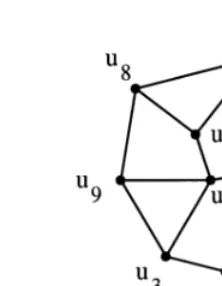
Fig. 1. Tiling
We will call T= (U; G) a tiling if
(1) P1; : : : ;PM are convex planar polygons
(2) [Pi]∩[Pj] is either empty or a common vertex or a common edge, i6=j,
(3) SM
i= 1[Pi] = [U].
Fig. 1 shows an example of a tiling T= (U; G) where
G= ((1;9;3);(3;4;5;6;1);(1;6;7;2);(1;2;8;9);(2;7;8)):
Note that condition (3) in the denition implies that the tiles [Pi] must cover a convex region of
the plane and that every point ui must belong to at least one polygon Pj. We think of G as the
‘topology’ of the tiling and the point sequence U as its ‘geometry’.
One kind of tiling T which occurs frequently in applications and which is of special interest to
us is when all its polygons have precisely three vertices (Kj= 3; j= 1; : : : ; M), in which case T
is a triangulation. It is well known in computational geometry (see e.g. [12]) that every point set
admits a Delaunay triangulation which has the property that the minimum angle of its triangles is maximized. Thus there exists at least one tiling of every point set. In general, a set of N points will admit an exponential number of tilings.
3. Compatible point sequences
Suppose we are given two sequences of N distinct planar points U0 and U1. By denition
U0 and U1 are points sets with a given correspondence, namely their common ordering. Such a
correspondence could be specied in a computer graphics application interactively by a user. Once a correpondence is established, it is easy to extend it to a mapping R2 → R2 by interpolating
between the corresponding points, using one of a variety of scattered data methods, such as radial basis functions. Perhaps the simplest method is a piecewise ane mapping : [U0]→[U1] over a
triangulationT0= (U0; G) ofU0. The triangulationT0, together with the triangulationT1= (U1; G)
induced onU1 byT0, denes an ane mapping between each of the corresponding pairs of triangles.
many triangulations, the rst problem is to nd a triangulation T0 of U0 which induces a (legal)
triangulation T1 on U1, said to be compatible with T0.
This combinatorial problem has been studied for point sets [1, 13] and polygons [17]. In short, we will say that two corresponding polygons, or corresponding point sets, are compatible if they admit a compatible triangulation. To determine whether two given point sets are compatible is believed to be NP-hard. It is possible to formulate many neccesary conditions for compatibility, but a nite set of sucient conditions has yet to be obtained. Souvaine and Wenger [17] show that if Steiner
points (extraneous points) are allowed, any two sets ofN points may be made compatible by adding O(N2) points, and there exist point sets of size N for whom at least (N2) points must be added in
order to obtain compatibility. Etzion and Rappoport [4] obtained similar results for the star-shaped compatibility of polygons (i.e. when the polygon is decomposed into star-shaped regions).
4. Morphable tilings
The question now arises, given two compatible triangulations or, more generally, tilings T0=
(U0; G) and T1= (U1; G), is this compatibility preserved when the tilings are morphed?
Denition 4.1. . A morph of two sequences of N distinct points U0 and U1 is any sequence
U= (u1; : : : ;uN) of continuous mappings ui: [0;1] → R2, i= 1; : : : ; N, such that ui(0) =u0i and
ui(1) =ui1.
A morph U generates an intermediate point sequence U(t) = (u1(t); : : : ;uN(t)) for each t∈(0;1).
We can think of each mapping ui as a parametric curve in R2 representing the path traced out
by the points ui(t) in moving from ui0 to u1i. If furthermore U0 andU1 are the vertex sets of a pair
of compatible tilings, we want to know whether the intermediate vertex sets U(t) induce ‘valid’ tilings.
Denition 4.2. We will say that two compatible tilings T0= (U0; G) and T1= (U1; G) are mor
-phableif there exists a morphU ofU0 andU1 such thatT(t) = (U(t); G) is a tiling for allt∈(0;1).
When trying to determine whether two compatible tilings are morphable, a natural candidate is the naive “straight line” or “linear” morph U dened by taking the weighted average
ui(t) = (1−t)ui0+tu 1
i; t∈[0;1]: (4.1)
If T0 andT1 are morphable with respect to this linear morph we say they are linearly morphable.
It turns out that not all compatible tilings are linearly morphable. In fact, if T0= (U0; G) is any
tiling withU0= (u0
as a rotation through of T0 in either a clockwise or anticlockwise direction, we could in this case
construct a ‘rotational’ morph by letting T0(t) be the rotation of T0 through an angle of t.
Lemma 4.3. Suppose T0= (U0; G) and T1= (U1; G)are two compatible tilings. If there are two
vertices u0
i and uj0 in U0; i6=j; such that
u0i =u1j and uj0=u1i; (4.2)
then T0 and T1 are not linearly morphable.
Proof. From Eqs. (4.1) and (4.2), we nd
which means that the point sequence U(1
2) = (u1( 1
2); : : : ;uN( 1
2)) contains two equal points and so
T(1
2) = (U( 1
2); G) cannot be a tiling.
We can apply Lemma 4.3 to show that two specic tilings with equal boundaries are not linearly morphable. Let T0= (U0; G) be the triangulation given by
and let T1= (U1; G) be the compatible triangulation dened by further letting
u11= (1;0); u12= (−1;0); u13= (2;−2); u41= (−2;2)
and u1
i =ui0, i= 5; : : : ;8. Since u10=u21 and u02=u11, Lemma 4.3 implies that T(12) is not a
triangu-lation and so T0 and T1 are not linearly morphable, as illustrated in Fig. 2.
In fact, even the more general morph U= (u1; : : : ;uN) given by
These counterexamples show that a more sophisticated method is needed in order to morph com-patible tilings.
5. Morphing by convex combinations
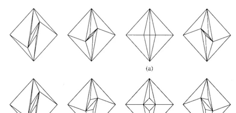
Fig. 2. (a) Linear morph. (b) Convex combination morph.
the interior vertices of two compatible tilingsT0 andT1 by convex combinations. We determine the
interior vertices of T(t) by averaging the convex combinations rather than the vertices themselves.
For notational convenience, let I be the set of indices i in {1; : : : ; N} such that uk
i is an interior
vertex of Tk and B the indices of boundary vertices, so that
I ∪B={1; : : : ; N} and I∩B=∅:
For each i∈I, let n(i)⊂{1;2; : : : ; N} denote the set of indices j∈ {1; : : : ; N} for which uk
j and uki
are neighbours.
We assume in this section that the boundaries of the tilings T0 and T1 are identical. Thus we
can dene a ‘constant’ morph for boundary points and we let ui(t) =u0i =ui1 for i∈B.
Next consider each interior vertex uk
i of Tk, k= 0;1. Since it clearly lies in the interior of the
convex hull of its neighbouring vertices it follows that it can be expressed as a convex combination of its neighbours. Thus, for each i∈I, there exist two sets of strictly positive real values k
ij∈R, j∈n(i), k∈ {0;1}, such that
X
j∈n(i)
kijujk=uik and X
j∈n(i)
kij= 1; k= 0;1: (5.1)
Then dening
ij(t) = (1−t)0ij+t 1
ij; t∈[0;1];
we clearly have ij(t)¿0 for each t and
X
j∈n(i)
We subsequently dene the |I|points ui(t)∈R2, i∈I, to be the solutions of the |I|linear equations
vertices and the solutions to the linear system (5.3) for interior ones.
Proof. It was shown in [5, 6] that the set of linear equations (5.3) has a unique solution, using the connectedness of the tiling and the weak diagonal dominance of the matrix.
Next we show that U is a morph. Since the values ij(t) depend continuously on t, it fol-lows from Eq. (5.3) that the mappings ui are continuous on [0;1]. Furthermore, due to the choice
of convex combinations in (5.1), the points uk
i for i∈I, k= 0;1, are the unique solutions to the
linear system (5.3) in the two cases t= 0;1, respectively. Therefore, ui(0) =ui0 and ui(1) =u1i
for i∈I and indeed all i= 1; : : : ; N, which establishes that U is a morph according to Denition 4.1.
Next we must check that T(t) = (U(t); G) is a tiling. It was also observed in [5, 6] that the set
of linear equations (5.3) is a simple generalization of those arising from the ‘barycentric mapping’ proposed by Tutte [19] for generating straight line drawings of planar graphs. In Tutte’s mapping the coecients ij(t) for xed i are constant and equal to 1=di where di is the valency ofui(t). Since the
theory in [19] (see also the prerequisite [18]) can be generalized to arbitrary convex combinations and the boundary polygon of U(t) is convex, it follows, as observed in [5], that T(t) is indeed a
tiling according to Denition 2.1. This establishes the condition of Denition 4.2.
In order to nd such a morph, we need to be able to express the interior vertices of a given tiling T= (U; G) as convex combinations of their neighbours. A little thought shows that each
interior vertex lies in the interior of the kernel of the star-shaped polygon formed by its neighbours. The following method for nding a suitable convex combination, proposed in [5], is based on this observation.
Suppose pandp1; : : : ;pd are distinct points inR2 such that P= (p1; : : : ;pd) is a star-shaped polygon
around the pointp which lies in the interior of the kernel of P. We construct a set of strictly positive values 1; : : : ; d satisfying
by averaging barycentric coordinates of a sequence of triangles covering p. Specically, for each
for all remaining j∈ {1; : : : ; d}, we have then expressed p as a convex combination
condition (5.4); see [5]. Without strict positivity of the coecients ij(t) in Eq. (5.3) there is no
obvious generalization of the theory in [19] and so we have no guarantee that T(t) in Theorem 5.1
is a valid tiling.
6. Morphing tilings with dierent boundaries
How do we extend the convex combination morph of the previous section to the general case where the boundaries of the two compatible tilings T0= (U0; G) and T1= (U1; G) are arbitrary?
We propose a solution in which we morph the two boundary polygons of T0 and T1 rst and
use the convex combination morph for interior vertices afterwards. Since the theory in [19] will only guarantee that T(t) is a genuine tiling if the boundary polygon of the point sequence U(t) is
convex, it is desirable to morph the two convex boundary polygons in such a way that convexity is preserved. Since we know of no method for doing this, we have implemented the following boundary morph, based on taking convex combinations of polar coordinates. This morph, suggested by Shapira and Rappoport [16] preserved convexity in all our numerical examples and it is easy to show that it at least preserves star-shapedness.
For notational convenience let us suppose that the boundary vertices are indexed uk
1; : : : ;ukn for k= 0;1 in an anticlockwise direction, where n=|B|. Thus, (u0
1; : : : ;u0n) and (u11; : : : ;un1) are the two
boundary polygons of T0 and T1. Since both boundaries are convex by denition, the two
By taking these ranges of angles we obtain a boundary morph which at least preserves
star-we dene a boundary morph by letting
ui(t) =u0(t) +ri(t)(cosi(t);sini(t)); i= 1; : : : ; n;
and it follows that
1(t)¡ 2(t)¡ · · ·¡ n(t)¡ 1(t) + 2:
7. Numerical examples
We have numerically computed both the linear morph and the convex combination morph for several pairs of compatible tilings. In the rst example, we take T0 and T1 to be triangulations
with identical boundaries as in example (4.3). Fig. 2(a) shows T0 (far left) andT1 (far right) and
triangulations T(i=4) for i= 1;2;3 generated by the linear morph (4.1). We can see that two of
the triangles in T(1
2) are degenerate, reecting the fact that the two vertices u1( 1
2) and u2( 1 2) are
coincident. Fig. 2(b) on the other hand, shows the result of applying the convex combination morph to T0 and T1.
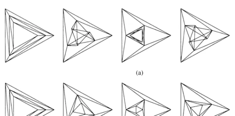
Figs. 3(a) and (b) show the results of the linear and convex combination morphs, respectively. Figs. 4(a) and (b) show the two morphs of compatible triangulations whose boundaries are dierent. The boundaries were morphed by taking convex combinations of polar coordinates as explained in Section 6.
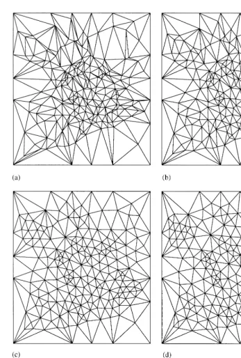
Fig. 5 shows two more complicated compatible triangulations T0 and T1 and their convex
combination morph at the valuest=1 3;
2
Fig. 3. (a) Linear morph. (b) Convex combination morph.
Fig. 4. (a) Linear morph. (b) Convex combination morph.
Bi-CGSTAB iterative method [20] applied to each of the two coordinates separately. The number of unknowns in this example is 187 since there are 187 interior vertices in the triangulation. In our implementation, for both t=1
3 and t= 2
3, the number of Bi-CGSTAB iterations in each coordinate
was between 21 and 24 and the total CPU time for computing each of the triangulations T(1
3) and
T(2
3) was 0.13 s. The triangulations T
0 andT1 were generated by mapping a surface triangulation
in R3 into the unit square using two dierent ‘parametrizations’ as in [5].
Fig. 5. (a)t= 0, (b) t=1 3, (c)t=
2
3, (d)t= 1.
8. Conclusion
We have described a morph based on convex combinations as an alternative to the standard linear one. Though the convex combination morph obviously requires more CPU time, an application of the kind in [9] requires only a small number of points, in which case computational speed is not crucial.
One question which naturally arises is whether the choice of the k
ij in (5.1) computed from Eq.
(5.5) has a signicant eect on the morph and the vertex paths. If the number of edges incident on each interior vertex in the tiling is minimal, i.e. three, then the k
ij determined by (5.5) are unique.
Otherwise it might be possible to make a choice which yields an optimal morph, for example in the sense that the vertex paths have minimal curvature.
It would also be interesting to characterize the pairs of compatible tilings which can be linearly morphed and which cannot. For example, the linear morph of the example in Fig. 5 also yields valid triangulations.
Finally, we would like a convexity-preserving morph of the two convex boundary polygons. A variety of methods [8, 14–16] have been proposed in the literature for morphing planar polygons, but none of them appear to preserve convexity. We plan to study this problem more closely in a forthcoming paper.
References
[1] B. Aronov, R. Seidel, D. Souvaine, On compatible triangulations of simple polygons, Comput. Geom. Theory Appl. 3 (1993) 27–35.
[2] T. Beier, S. Neely, Feature-based image metamorphosis, Comput. Graphics 26 (1992) 35–42. [3] S. Cohen, G. Elber, R. Bar-Yehuda, Matching of freeform curves, CAD 29 (1997) 369–378.
[4] M. Etzion, A. Rappoport, On compatible star decompositions of star polygons, IEEE Trans. Visual and Comput Graphics 3 (1997) 87–95.
[5] M.S. Floater, Parametrization and smooth approximation of surface triangulations, Comp. Aided Geom. Des. 14 (1997) 231–250.
[6] M.S. Floater, Parametric tilings and scattered data approximation, Internat. J. Shape Modeling, to appear. [7] K. Fujimura, M. Makarov, Foldover-free image warping, Graphical Models Image Process. 60 (1998) 100–111. [8] E. Goldstein, C. Gotsman, Polygon morphing using a multiresolution approach, Proc. Graphics Interface, 1995. [9] R. Gore, K. Garrett, R. Schlecht, Virtual Neanderthals, National Geographic 189 (1996) 15.
[10] T. He, S. Wang, A. Kaufman. Wavelet-based volume morphing, Proc. of Visualization ’94, IEEE Computer Society, 1994.
[11] J. Hughes, Scheduled Fourier volume morphing, Comput. Graphics 26 (1992) 43–46. [12] F.P. Preparata, M.I. Shamos, Computational Geometry, Springer, New York, 1985.
[13] A. Saalfeld, Joint triangulations and triangulation maps, Proc. 3rd Ann. ACM Sympos. Comput. Geom., 1987, pp. 195–204.
[14] T.W. Sederberg, E. Greenwood, A physically based approach to 2D shape blending, Comput. Graphics 26 (1992) 25–34.
[15] T.W. Sederberg, P. Gao, G. Wang, H. Mu, 2D shape blending: an intrinsic solution to the vertex path problem, Comput. Graphics 27 (1993) 15–18.
[17] D. Souvaine, R. Wenger, Constructing piecewise linear homeomorphisms, DIMACS Technical Report 94-52, Rutgers University, December 1994.
[18] W.T. Tutte, Convex representations of graphs, Proc. London Math. Soc. 10 (1960) 304–320. [19] W.T. Tutte, How to draw a graph, Proc. London Math. Soc. 13 (1963) 743–768.